绘图工具与实例:seaborn
2 Seaborn
该库对Matplotlib进行了更高级的封装,使得用户可以在少量代码下绘制出复杂的图形。
2.1 图类型
Seaborn提供的可绘制图类型包括统计关系型、数据分布型、分类数据型、回归模型分析型和多子图网格型。
2.1.1 关系型
2.1.1.1 scatterplot()
seaborn.scatterplot(data=None, *, x=None, y=None, hue=None, size=None, style=None, palette=None, hue_order=None, hue_norm=None, sizes=None, size_order=None, size_norm=None, markers=True, style_order=None, legend='auto', ax=None, **kwargs)
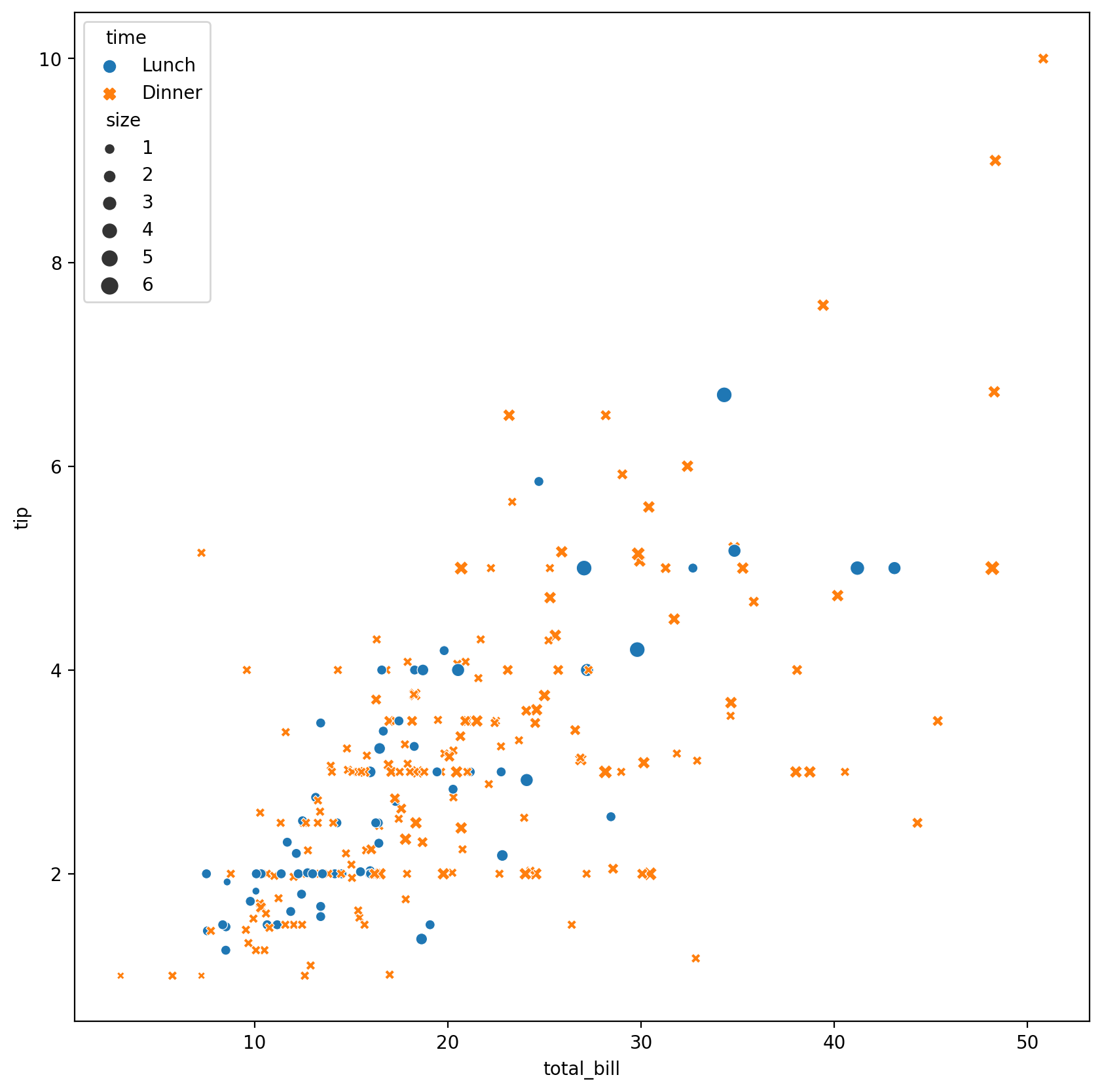
data绘图源数据,可以为pandas.DataFrame,numpy.ndarray等序列或映射x、y确定两坐标轴对应的变量hue指定某一变量,其不同值对应图中的不同颜色size指定某一变量,其不同值对应图中不同点的大小style指定某一变量,其不同值对应图中的不同模式(如实线与虚线)palette指定将hue中元素到不同颜色之间的映射sizes确定不同size选用的方案markers确定不同点类型的选用方案legend"auto","brief","full", 或False**kwargs其他传给matplotlib.pyplot.scatter()函数的关键字参数
以下是官网的使用例:
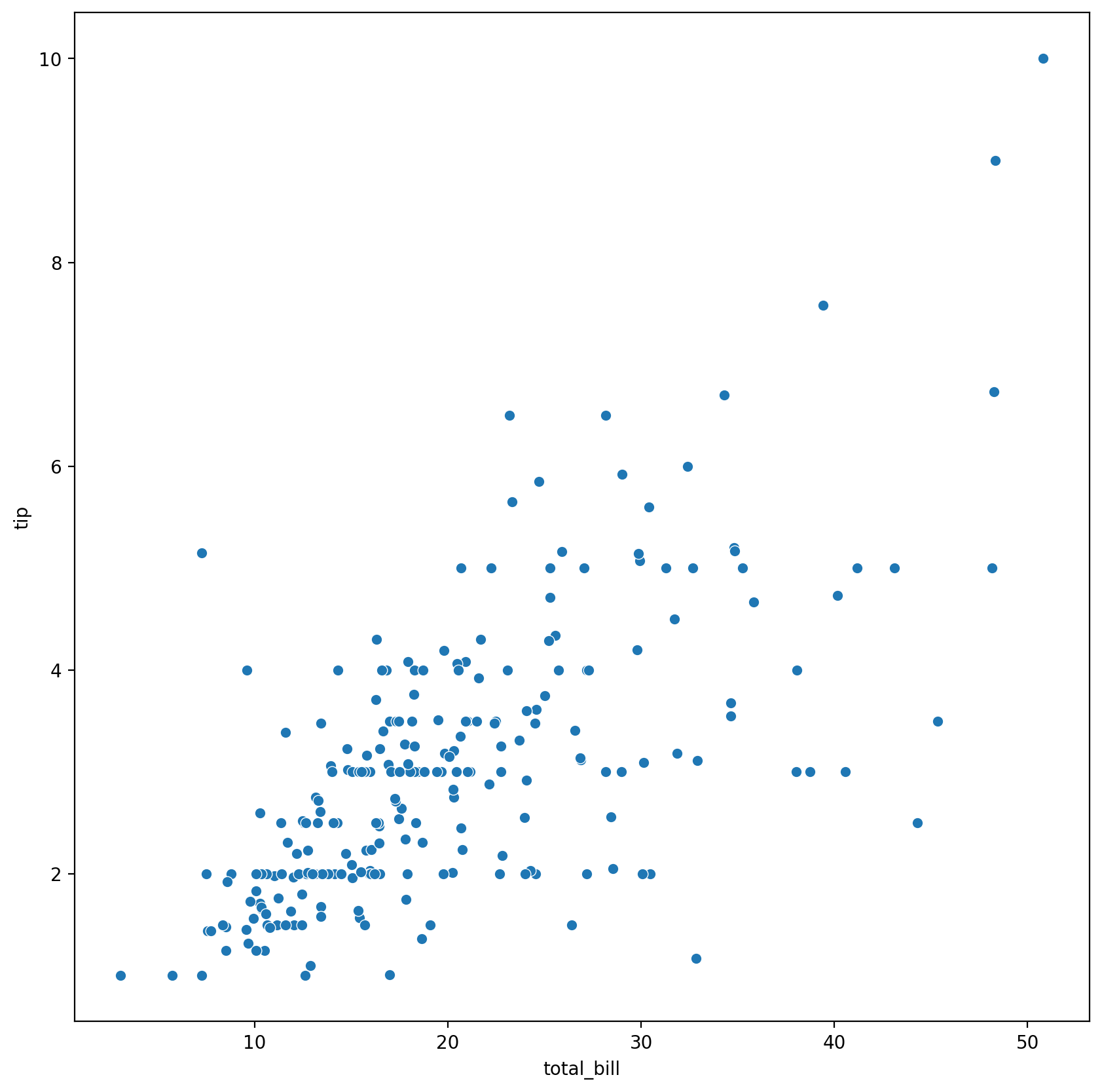
import seaborn as sns# 一些方便的设置def plot(plot_func, fig_size, **kwargs): plt.figure(figsize=fig_size, dpi=200) ax = plt.subplot(111) plot_func(ax=ax, **kwargs) plt.show()# 加载数据tips = sns.load_dataset("tips")# 这个数据集一共有七列,即# | total_bill | tip | sex | smoker | day | time | size |# 不指定其他参数plot(sns.scatterplot, (10, 10), data=tips, x="total_bill", y="tip") |
# 指定hue、style、sizeplot(sns.scatterplot, (10, 10), data=tips, x="total_bill", y="tip", hue="time", style="time", size="size") |
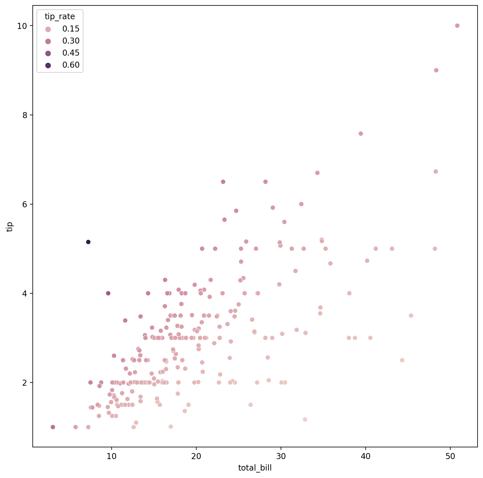
# 指定hue为数值(numerical)而非分类(categorical)类型plot(sns.scatterplot, (10, 10), data=tips, x="total_bill", y="tip", hue=tips.eval("tip / total_bill").rename("tip_rate") ) |
2.1.1.2 relplot()
seaborn.relplot(data=None, *, x=None, y=None, hue=None, size=None, style=None, units=None, row=None, col=None, col_wrap=None, row_order=None, col_order=None, palette=None, hue_order=None, hue_norm=None, sizes=None, size_order=None, size_norm=None, markers=None, dashes=None, style_order=None, legend='auto', kind='scatter', height=5, aspect=1, facet_kws=None, **kwargs)
units分类变量的指标,一般用于绘制多次重复实验的结果row、col用于定义不同行和列的对应指标dashes定义线型kind选择线图或散点图height每个子图的高(inch)aspect每个子图的宽高比,width = aspect * heightfacet_kw传入FacetGrid的关键字参数
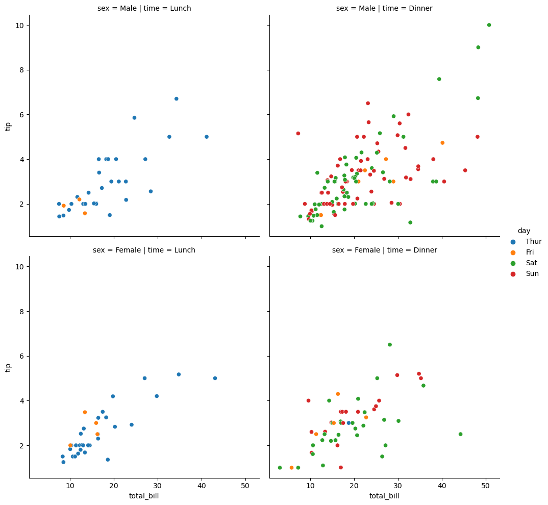
# 指定hue,并分别指定行和列sns.relplot(data=tips, x="total_bill", y="tip", hue="day", col="time", row="sex" ) |
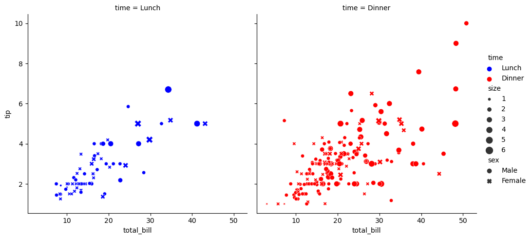
# 指定hue、col和rowsns.relplot(data=tips, x="total_bill", y="tip", col="time", hue="time", size="size", style="sex", palette=["b", "r"], sizes=(10, 100) ) |
2.1.1.3 lineplot()
seaborn.lineplot(data=None, *, x=None, y=None, hue=None, size=None, style=None, units=None, palette=None, hue_order=None, hue_norm=None, sizes=None, size_order=None, size_norm=None, dashes=True, markers=None, style_order=None, estimator='mean', errorbar =('ci', 95), n_boot=1000, seed=None, orient='x', sort=True, err_style='band', err_kws=None, legend='auto', ci='deprecated', ax=None, **kwargs)
estimator估计方法,类型为callable或None,用于估计图线在某一处的值errorbar选择对应的errorbar方法,或传入一个元组n_boot计算置信区间时所使用的自助次数seed自助法所使用的随机种子orient目标函数的独立变量sort对x或y变量进行排序
flights = sns.load("flights")flights.head() |
| year | month | passengers | |
|---|---|---|---|
| 0 | 1949 | Jan | 112 |
| 1 | 1949 | Feb | 118 |
| 2 | 1949 | Mar | 132 |
| 3 | 1949 | Apr | 129 |
| 4 | 1949 | May | 121 |
may_flights = floghts.query("month == 'May'")may_flights.head() |
| year | month | passengers | |
|---|---|---|---|
| 4 | 1949 | May | 121 |
| 16 | 1950 | May | 125 |
| 28 | 1951 | May | 172 |
| 40 | 1952 | May | 183 |
| 52 | 1953 | May | 229 |
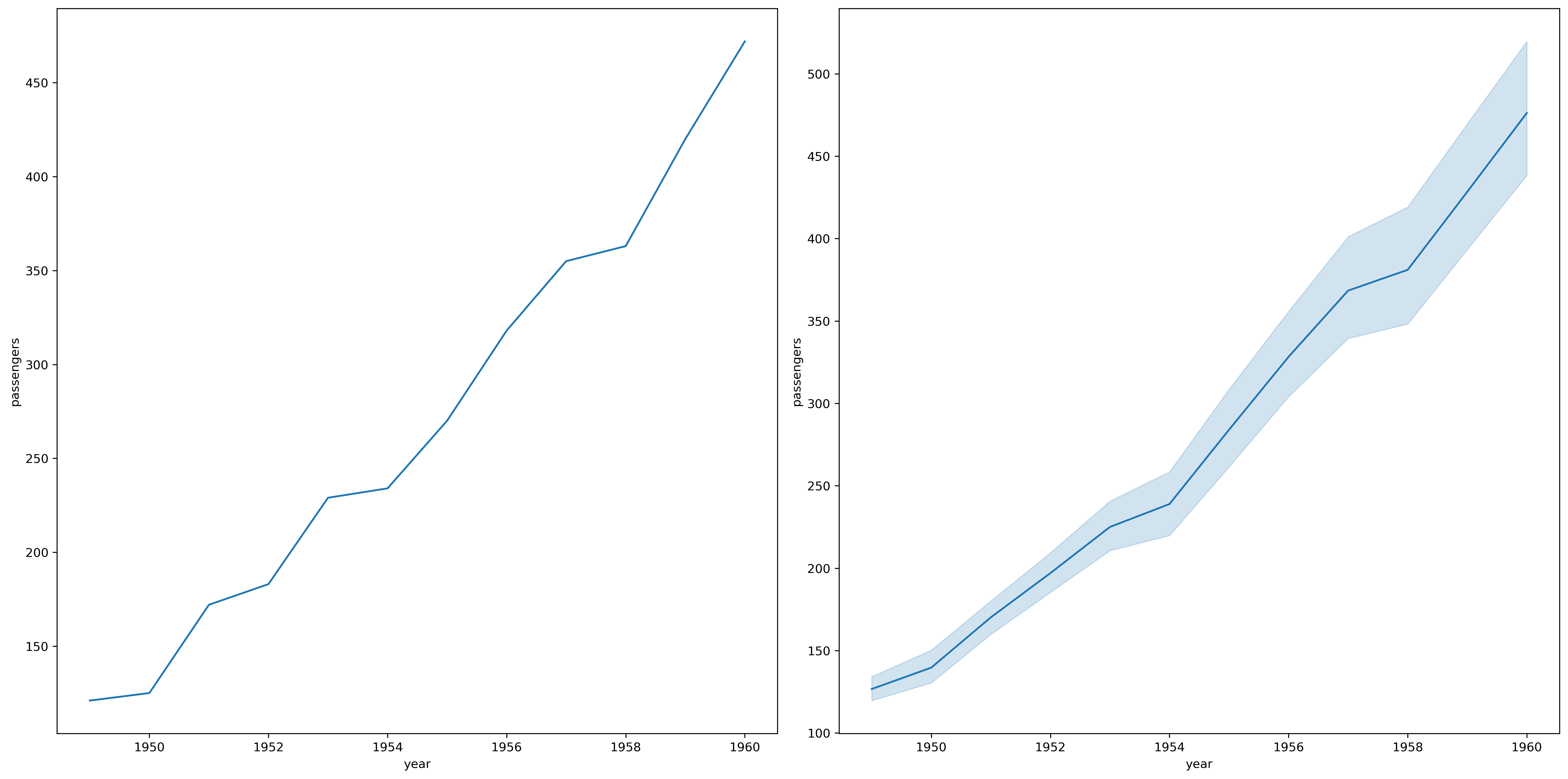
plt.figure(dpi=300, figsize=(18, 9))ax = plt.subplot(121)sns.lineplot(data=may_flights, x="year", y="passengers", ax=ax)ax = plt.subplot(122)sns.lineplot(data=flights, x="year", y="passengers", ax=ax)plt.tight_layout() |
flights_wide = flights.pivot("year", "month", "passengers")flights_wide.head() |
| month | Jan | Feb | Mar | Apr | May | Jun | Jul | Aug | Sep | Oct | Nov | Dec |
|---|---|---|---|---|---|---|---|---|---|---|---|---|
| year | ||||||||||||
| 1949 | 112 | 118 | 132 | 129 | 121 | 135 | 148 | 148 | 136 | 119 | 104 | 118 |
| 1950 | 115 | 126 | 141 | 135 | 125 | 149 | 170 | 170 | 158 | 133 | 114 | 140 |
| 1951 | 145 | 150 | 178 | 163 | 172 | 178 | 199 | 199 | 184 | 162 | 146 | 166 |
| 1952 | 171 | 180 | 193 | 181 | 183 | 218 | 230 | 242 | 209 | 191 | 172 | 194 |
| 1953 | 196 | 196 | 236 | 235 | 229 | 243 | 264 | 272 | 237 | 211 | 180 | 201 |
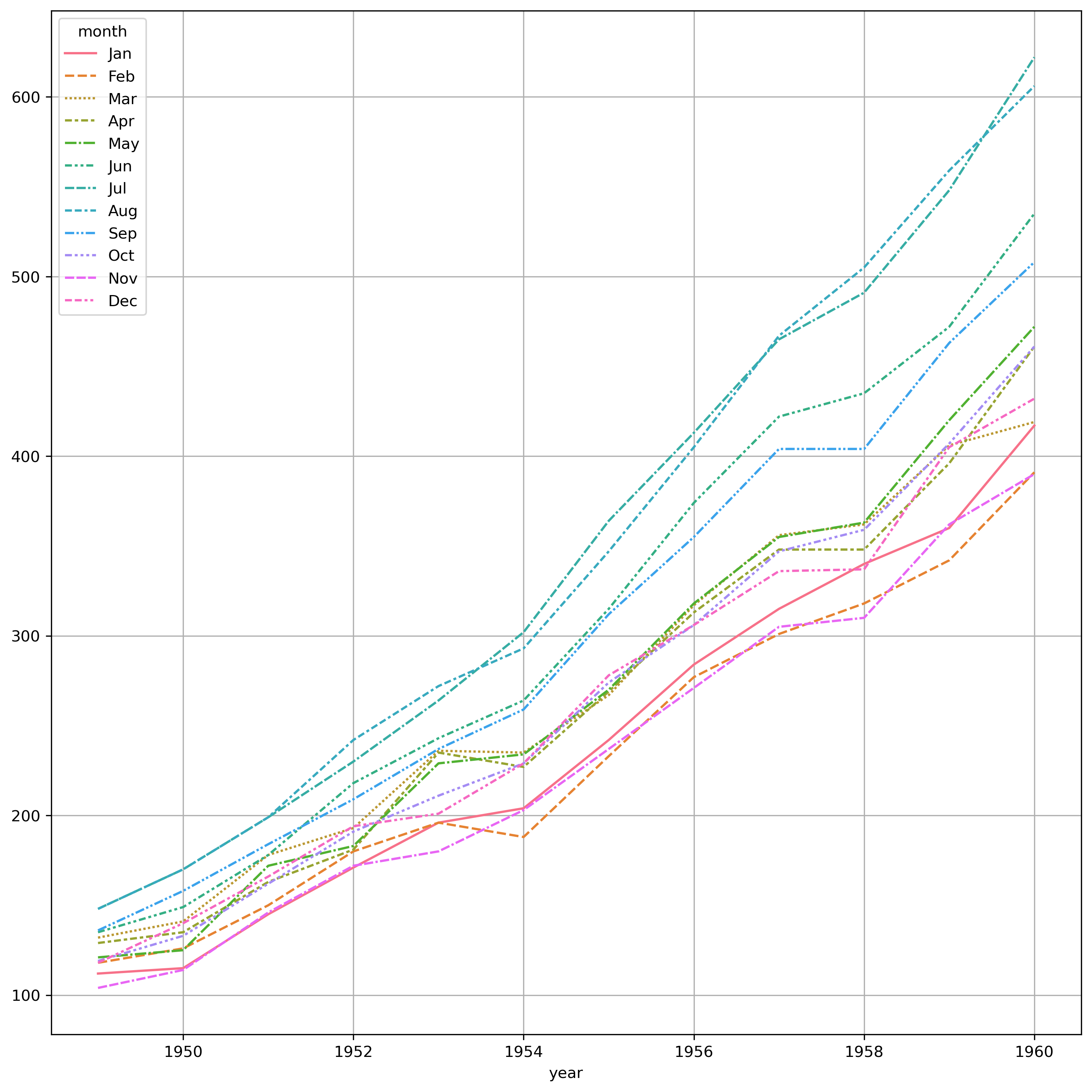
plt.figure(dpi=300, figsize=(12, 12))sns.lineplot(data=flights_wide)plt.grid() |
fmri = sns.load_dataset("fmri")plt.figure(dpi=300, figsize=(16, 16))plt.subplot(2, 2, 1)sns.lineplot(data=fmri, x="timepoint", y="signal", hue="event")plt.subplot(2, 2, 2)sns.lineplot(data=fmri, x="timepoint", y="signal", hue="region", style="event")plt.subplot(2, 2, 3)sns.lineplot(data=fmri, x="timepoint", y="signal", hue="region", style="event", markers=True, dashes=False)plt.subplot(2, 2, 4)sns.lineplot(data=fmri, x="timepoint", y="signal", hue="region", style="event", markers=True, err_style="bars") |
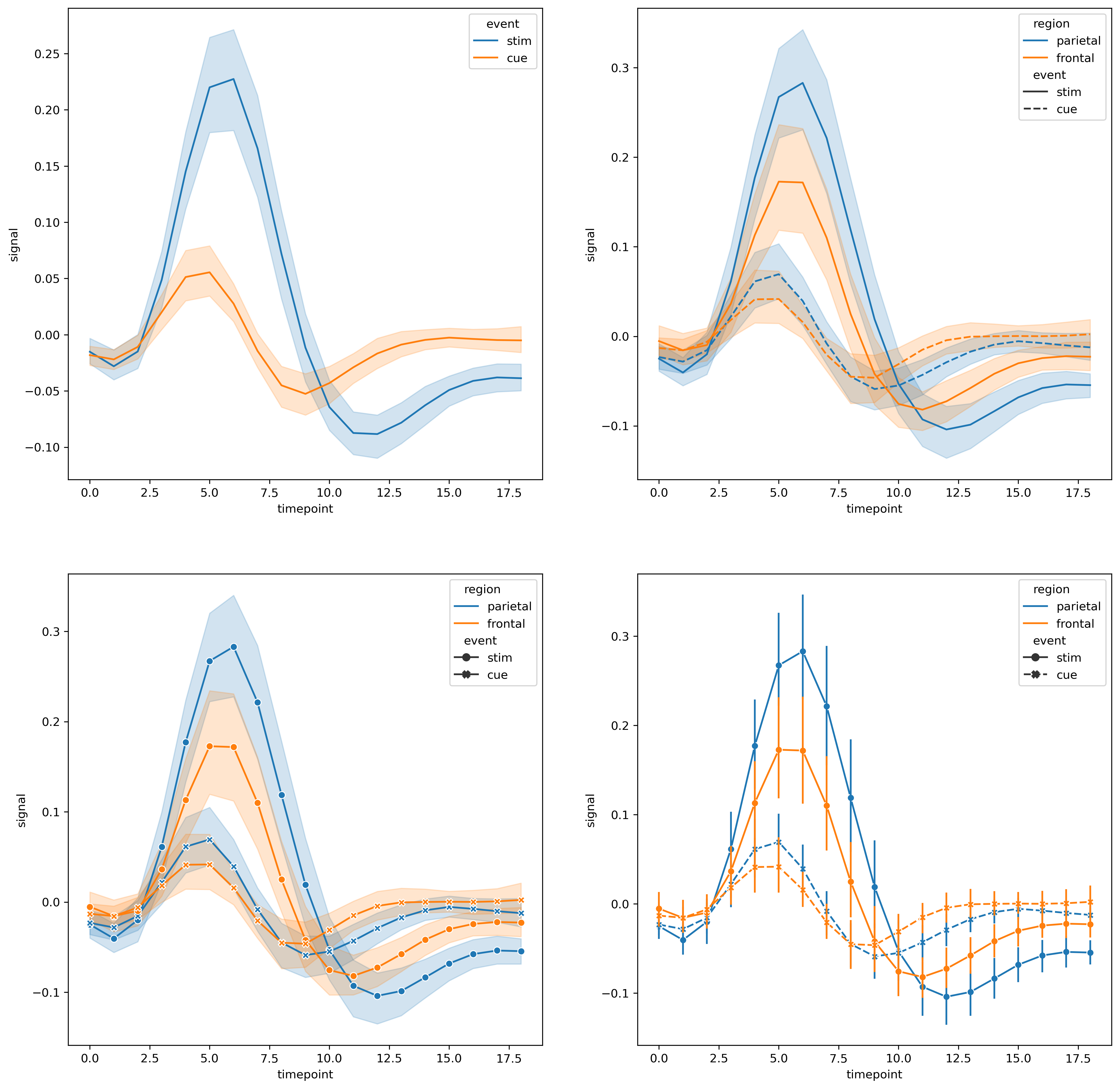
值得注意的是,笔者使用的seaborn版本和所查文档的版本不同,lineplot函数中没有errorbar参数,而是error_style。
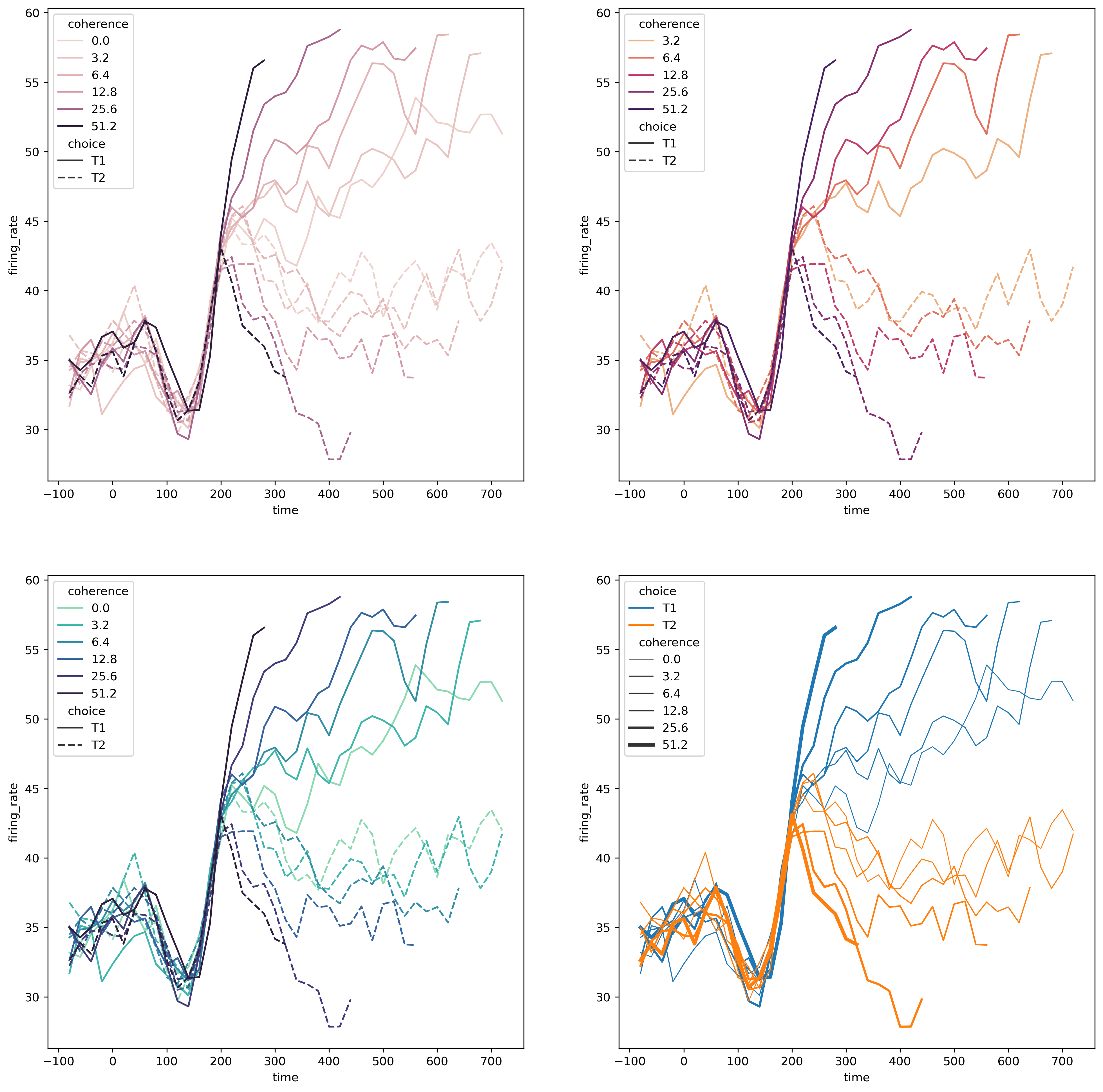
import matplotlib as mpldots = sns.load_dataset("dots").query("align == 'dots'")plt.figure(dpi=300, figsize=(16, 16))plt.subplot(2, 2, 1)sns.lineplot(data=dots, x="time", y="firing_rate", hue="coherence", style="choice")plt.subplot(2, 2, 2)sns.lineplot(data=dots.query("coherence > 0"), x="time", y="firing_rate", hue="coherence", style="choice", palette="flare", hue_norm=mpl.colors.LogNorm())plt.subplot(2, 2, 3)palette = sns.color_palette("mako_r", 6)sns.lineplot(data=dots, x="time", y="firing_rate", hue="coherence", style="choice", palette=palette)plt.subplot(2, 2, 4)sns.lineplot(data=dots, x="time", y="firing_rate", size="coherence", hue="choice", legend="full") |
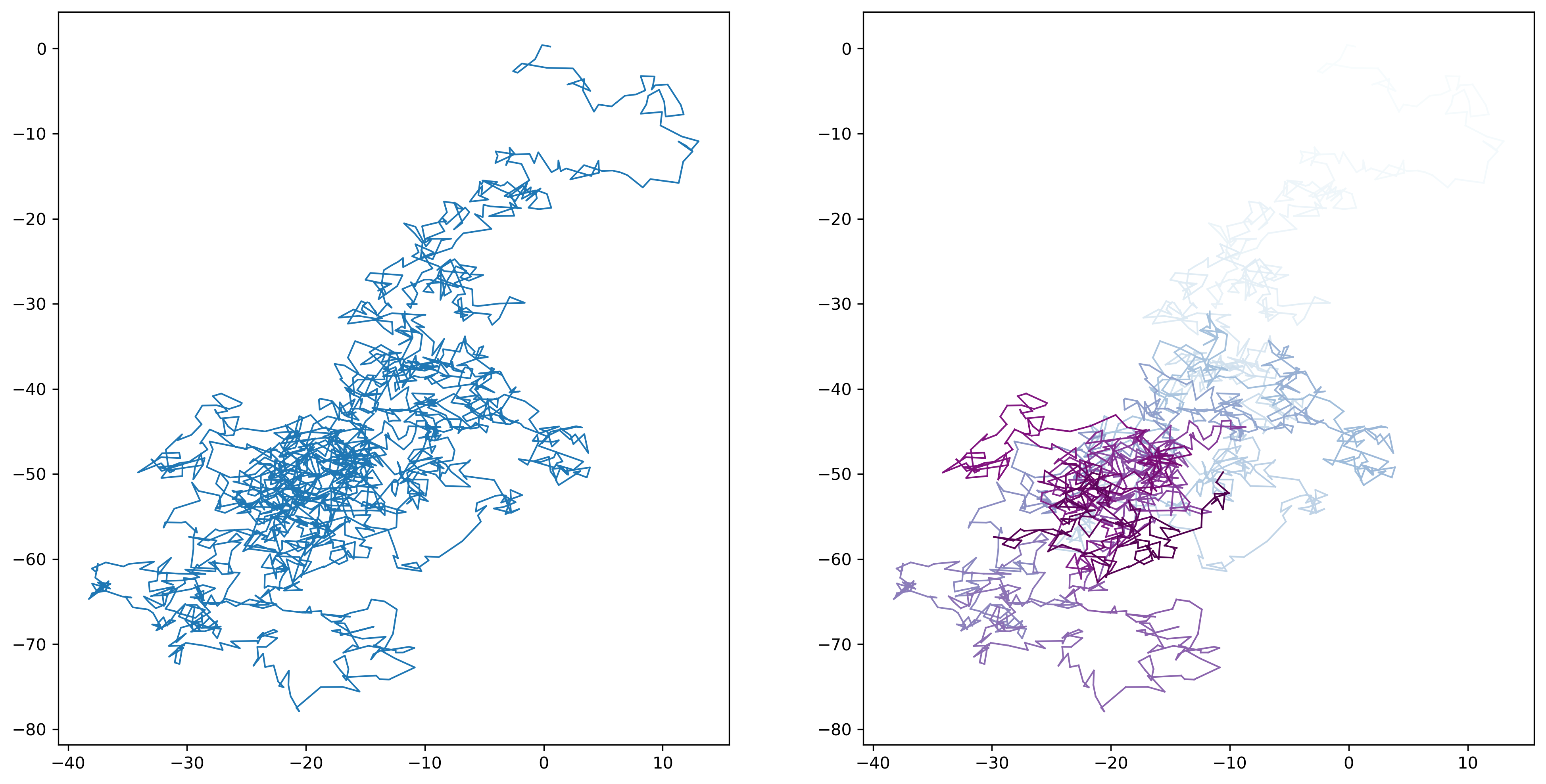
在默认情况下,seaborn会对输入的x变量进行排序,在一些特定情况下,我们并不希望进行这样的操作。下面就是一个例子
from tqdm import tqdmITER_NUM = 2000x, y = np.random.normal(size=(2, ITER_NUM)).cumsum(axis=1)plt.figure(dpi=300, figsize=(16, 8))# 直接绘制ax = plt.subplot(121)sns.lineplot(x=x, y=y, sort=False, lw=1, ax=ax)# 添加渐变颜色以显示轨迹的新旧ax = plt.subplot(122)hue = np.linspace(0, 5, ITER_NUM) / 5 + 1e-5for i in tqdm(range(0, ITER_NUM)): sns.lineplot(x=x[i:i+2], y=y[i:i+2], sort=False, lw=1, color=plt.get_cmap("BuPu")(hue[i]), legend=False, ax=ax) |
2.1.2 数据分布型
2.1.2.1 displot()
绘制分布图的函数。
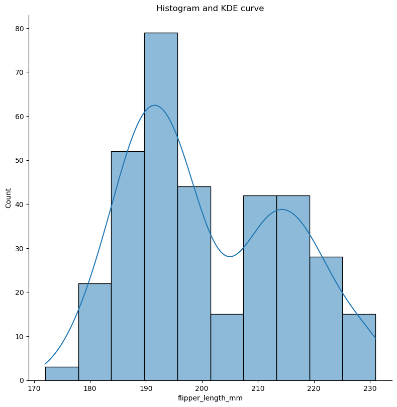
penguins = sns.load_dataset("penguins")sns.displot(data=penguins, x="flipper_length_mm", kde=True, facet_kws={"size":8})plt.xlabel("flipper_length_mm")plt.title("Histogram and KDE curve") |
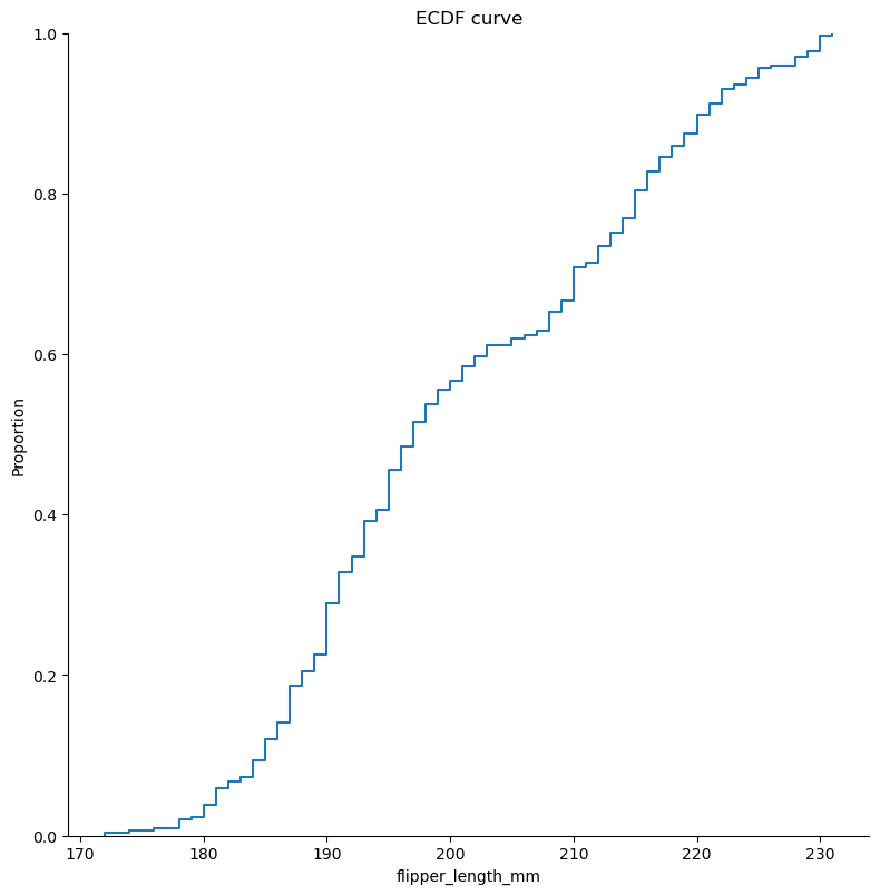
sns.displot(data=penguins, x="flipper_length_mm", kind="ecdf", facet_kws={"size":8})plt.xlabel("flipper_length_mm")plt.title("ECDF curve") |
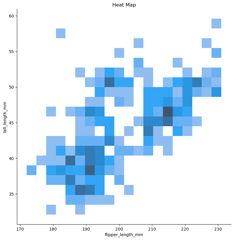
sns.displot(data=penguins, x="flipper_length_mm", y="bill_length_mm", bins=20 , height=8)plt.title("Heat Map") |
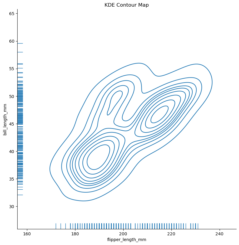
sns.displot(data=penguins, x="flipper_length_mm", y="bill_length_mm", height=8, kind="kde", rug=True)plt.title("KDE Contour Map") |
2.1.2.2 histpot()
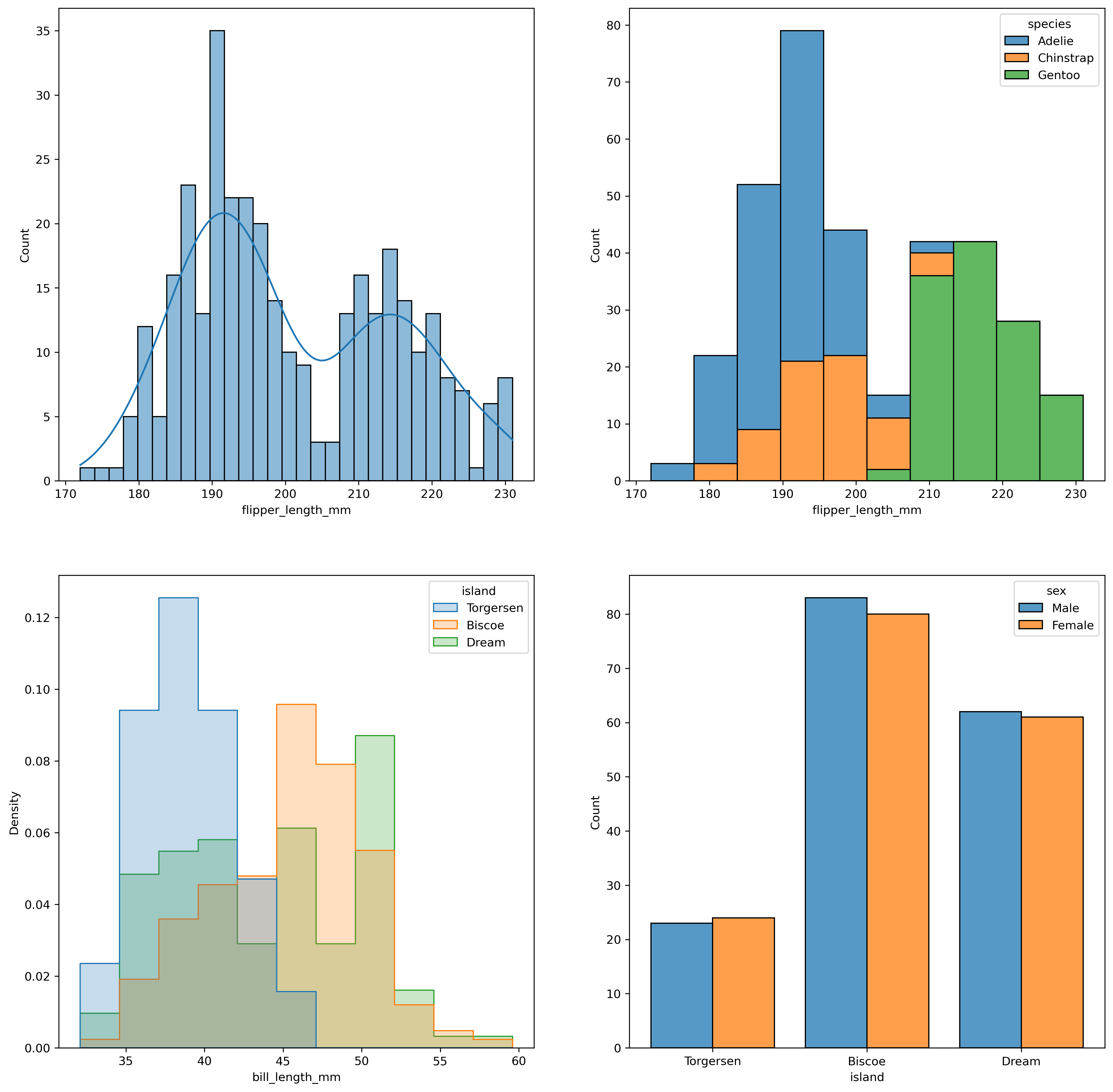
penguins = penguins = sns.load_dataset("penguins")plt.figure(figsize=(16, 16), dpi=300)plt.subplot(2, 2, 1)# 还可以使用 binwidth 间接控制 bins 的数量sns.histplot(data=penguins, x="flipper_length_mm", bins=30, kde=True)plt.subplot(2, 2, 2)# 使用 hue 区分不同的分布,并可以指定 multiple 为 "stack" 避免遮挡的情况sns.histplot(data=penguins, x="flipper_length_mm", hue="species", multiple="stack")plt.subplot(2, 2, 3)# 指定 common_norm 将所有数据进行归一化sns.histplot( penguins, x="bill_length_mm", hue="island", element="step", stat="density", common_norm=False,)plt.subplot(2, 2, 4)# 在离散的数据下绘制条形图sns.histplot(data=penguins, x="island", hue="sex", multiple="dodge", shrink=.8) |
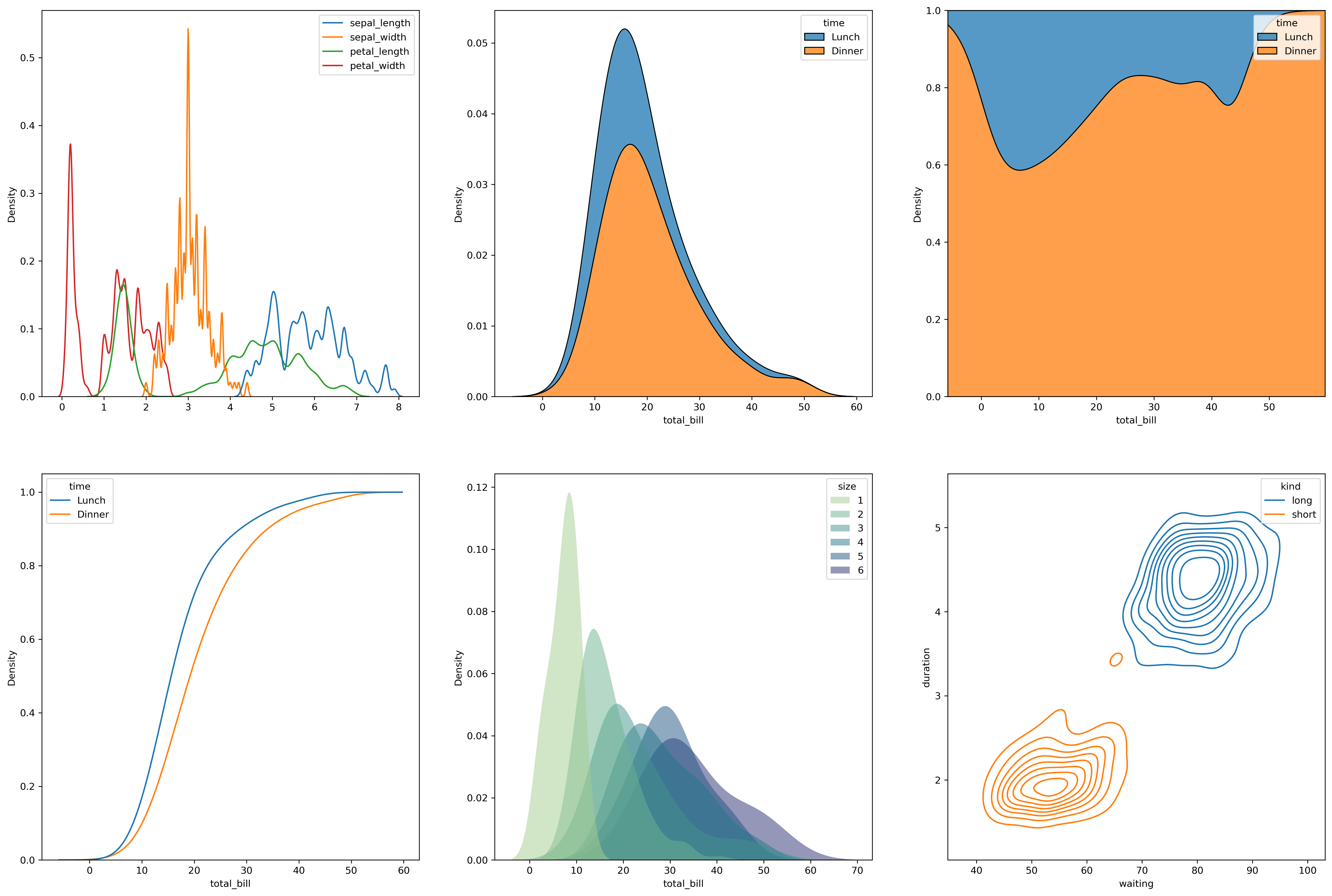
2.1.2.3 kdeplot()
iris = sns.load_dataset("iris")tips = sns.load_dataset("tips")geyser = sns.load_dataset("geyser")plt.figure(dpi=300, figsize=(24, 16))plt.subplot(2, 3, 1)# 绘制多个分布密度估计曲线并调整平滑带宽sns.kdeplot(data=iris, bw_adjust=.2)plt.subplot(2, 3, 2)# 堆叠多个分布估计曲线sns.kdeplot(data=tips, x="total_bill", hue="time", multiple="stack")plt.subplot(2, 3, 3)# 归一化多个分布估计曲线sns.kdeplot(data=tips, x="total_bill", hue="time", multiple="fill")plt.subplot(2, 3, 4)# 绘制多个累积分布估计曲线sns.kdeplot( data=tips, x="total_bill", hue="time", cumulative=True, common_norm=False, common_grid=True)plt.subplot(2, 3, 5)# 使用数值类型的 huesns.kdeplot( data=tips, x="total_bill", hue="size", fill=True, common_norm=False, palette="crest", alpha=.5, linewidth=0,)plt.subplot(2, 3, 6)# 绘制多个二维分布的等高线图,并设置参数sns.kdeplot( data=geyser, x="waiting", y="duration", hue="kind", levels=10, thresh=.1,) |
2.1.2.4 ecdfplot()
上文中已有使用cedfplot绘制的例子,在此不再赘述。
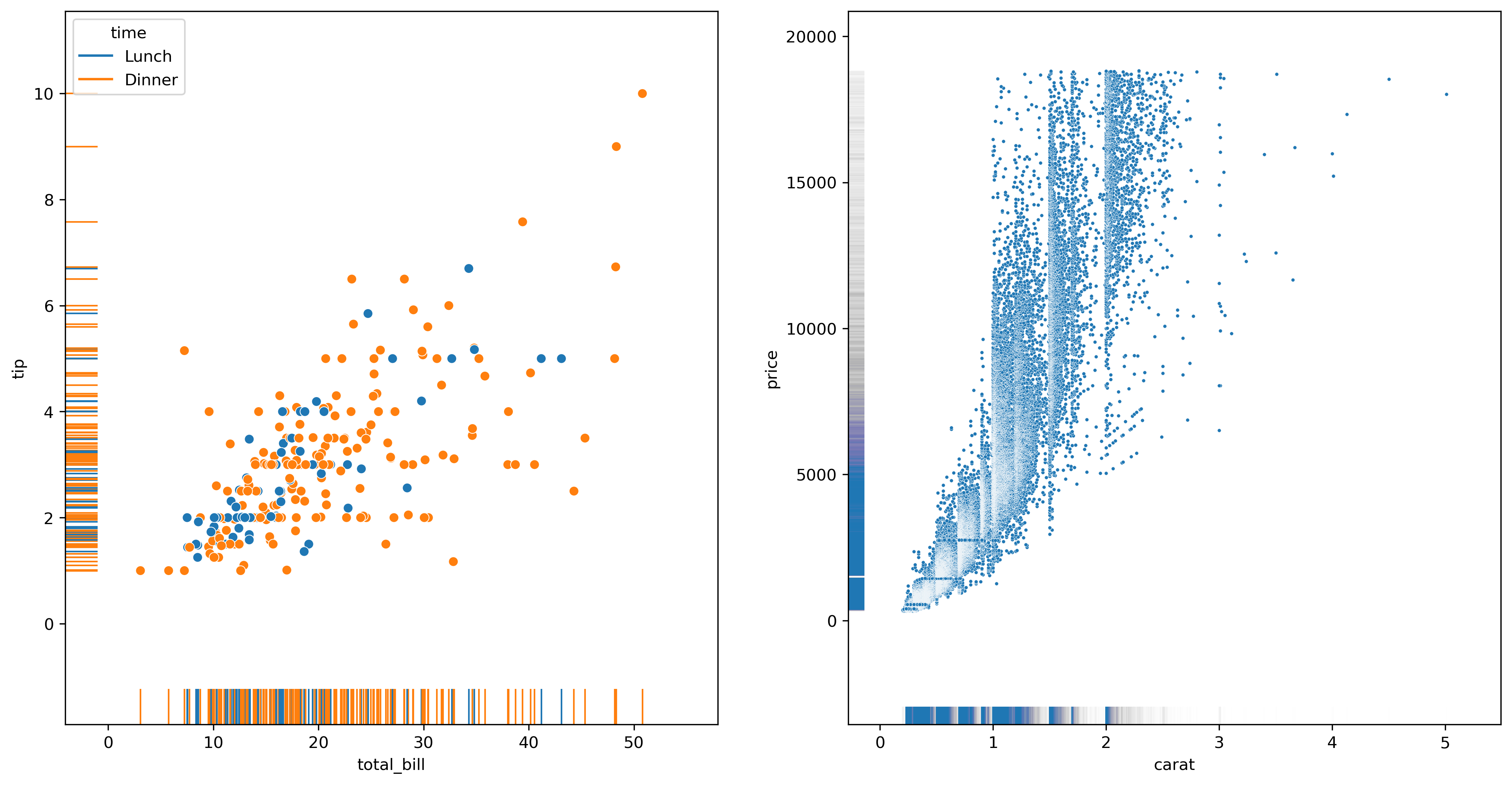
2.1.2.5 rugplot()
plt.figure(dpi=300, figsize=(16, 8))plt.subplot(1, 2, 1)# rugplot 往往是在scatterplot的基础之上绘制的sns.scatterplot(data=tips, x="total_bill", y="tip", hue="time")sns.rugplot(data=tips, x="total_bill", y="tip", hue="time", height=0.05)plt.subplot(1, 2, 2)# 在面对大数据集时,需要适当的将线条粗细降低,将线条透明度调高diamonds = sns.load_dataset("diamonds")sns.scatterplot(data=diamonds, x="carat", y="price", s=5)sns.rugplot(data=diamonds, x="carat", y="price", lw=1, alpha=.005) |
2.1.3 分类数据型
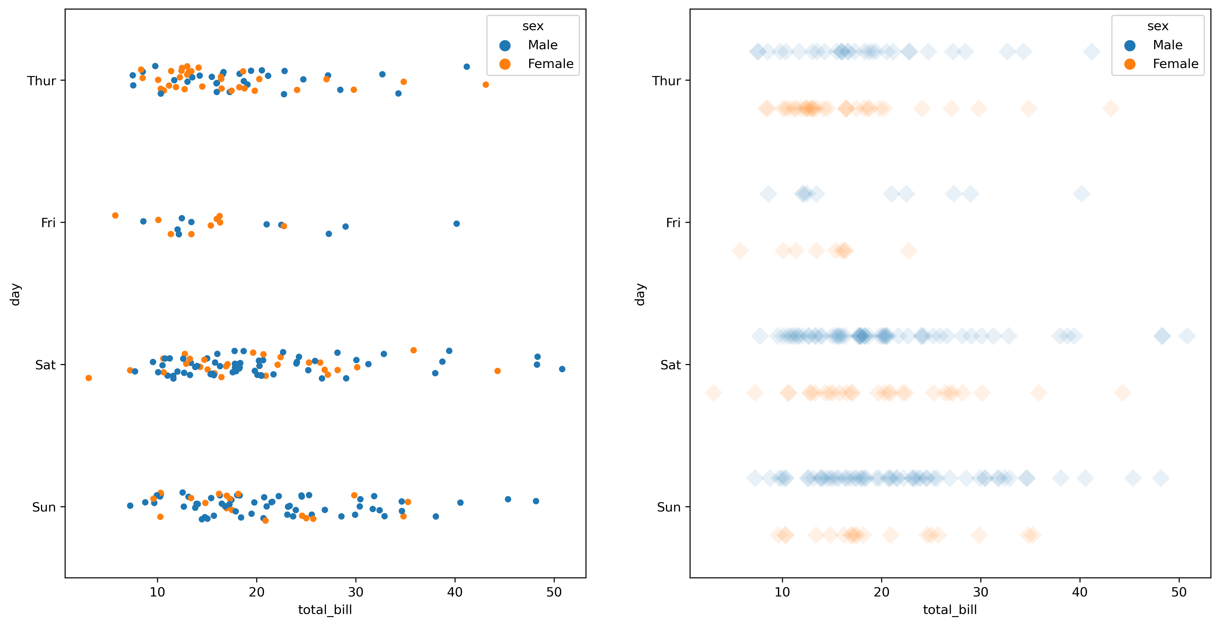
2.1.3.1 stripplot()
plt.figure(dpi=300, figsize=(16, 8))# 添加类别plt.subplot(1, 2, 1)sns.stripplot(data=tips, x="total_bill", y="day", hue="sex")# 设置 dodge 为 True 以做到不同 hue 的分离,调整 jitter 为 False 使得数据点纵向不堆叠plt.subplot(1, 2, 2)sns.stripplot(data=tips, x="total_bill", y="day", hue="sex", dodge=True, jitter=False , marker='D', alpha=.1, s = 10) |
2.1.3.2 swarmplot()
2.1.3.3 boxplot()
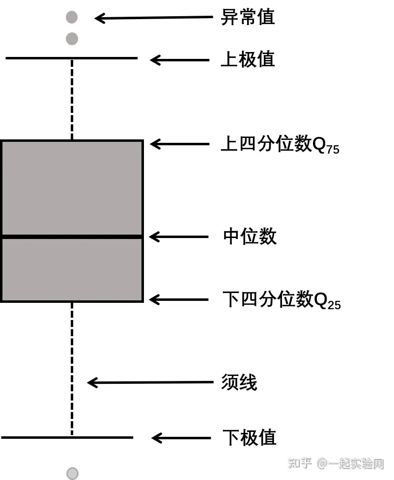
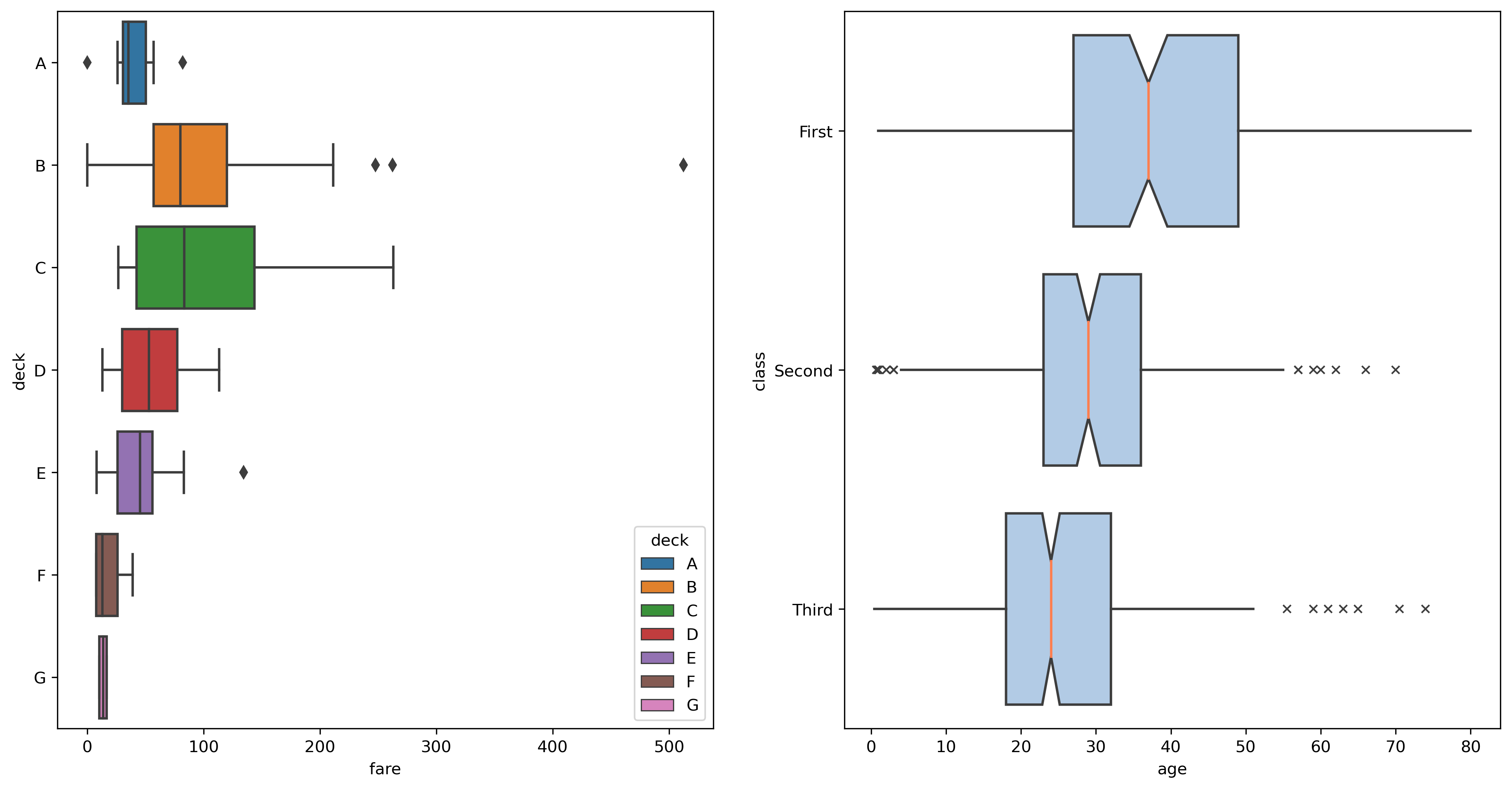
箱线图可以显示数据的主要统计量,如中位数、四分位数、离群值等,如下图所示。
df = sns.load_dataset("titanic")plt.figure(dpi=300, figsize=(16, 8))plt.subplot(1, 2, 1)sns.boxplot(data=df, x="fare", y="deck", hue="deck", dodge=False)plt.subplot(1, 2, 2)sns.boxplot( data=df, x="age", y="class", notch=True, # 将箱线图类型设置为“葫芦”的形状 showcaps=False, # 是否显示头尾两条垂直线 flierprops={"marker": "x"}, # 设置离群值点属性 boxprops={"facecolor": (.4, .6, .8, .5)}, # 设置颜色,分别为 RGB 和透明度 medianprops={"color": "coral"}, # 设置中位数属性) |
2.1.3.4 violinplot()
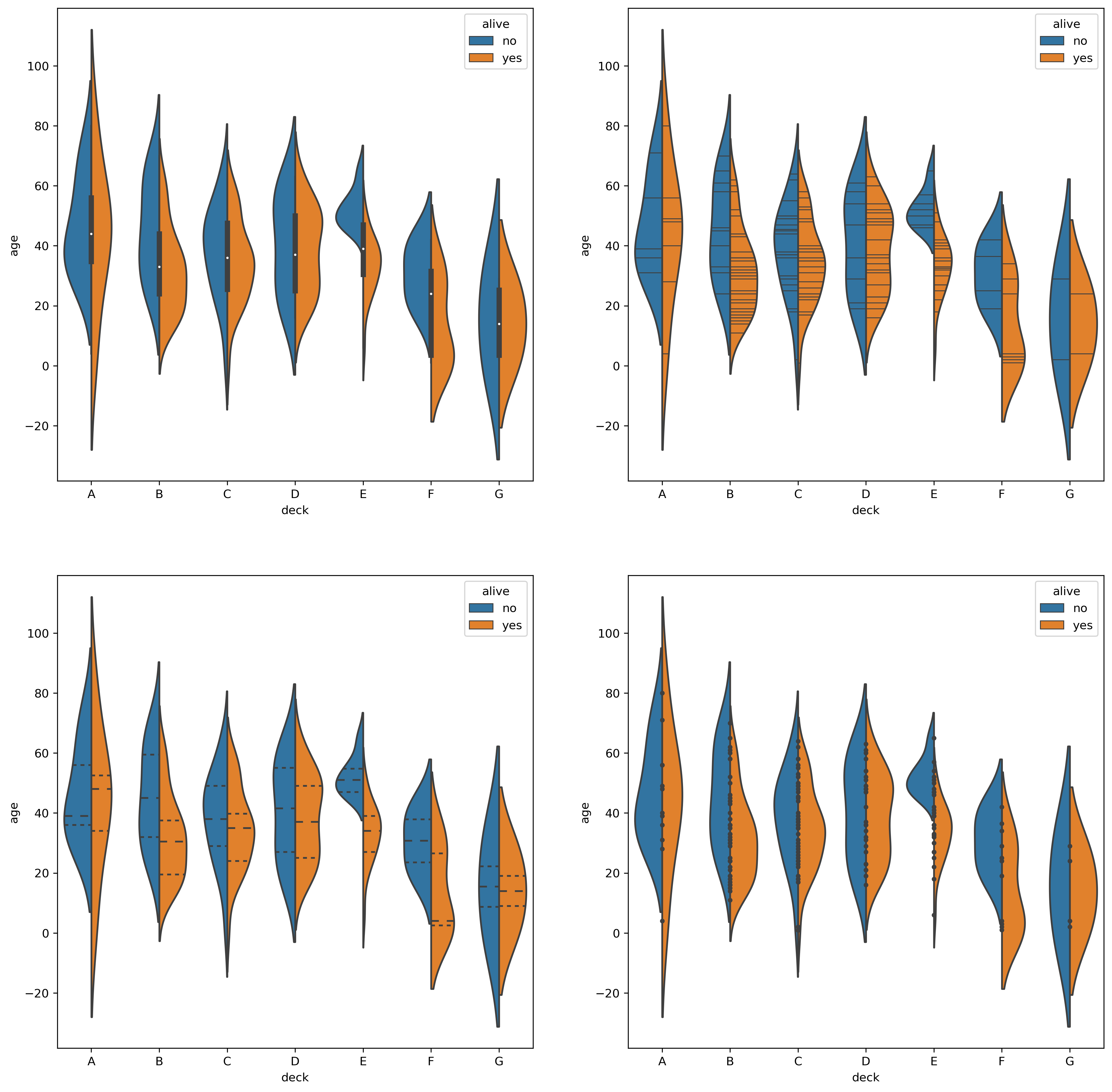
提琴图除了拥有箱线图的优点以外还可以很好的反应数据的分布特征
df = sns.load_dataset("titanic")plt.figure(dpi=300, figsize=(16, 16))plt.subplot(2, 2, 1)sns.violinplot(data=df, x="deck", y="age", hue="alive", split=True)# 画密度线plt.subplot(2, 2, 2)sns.violinplot(data=df, x="deck", y="age", hue="alive", split=True, inner="stick")# 四分位数plt.subplot(2, 2, 3)sns.violinplot(data=df, x="deck", y="age", hue="alive", split=True, inner="quartile")# 画独立实验点 (Individual Observartions)plt.subplot(2, 2, 4)sns.violinplot(data=df, x="deck", y="age", hue="alive", split=True, inner="point") |
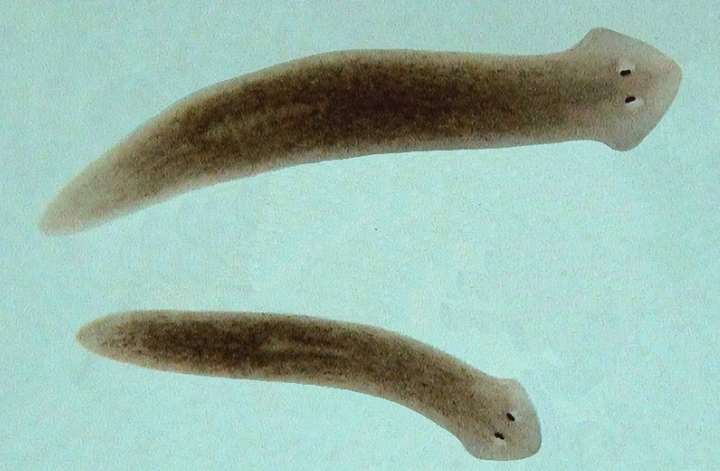
p.s. 这玩意儿感觉有点像涡虫(下图,还怪可爱的)
2.1.3.5 boxenplot()
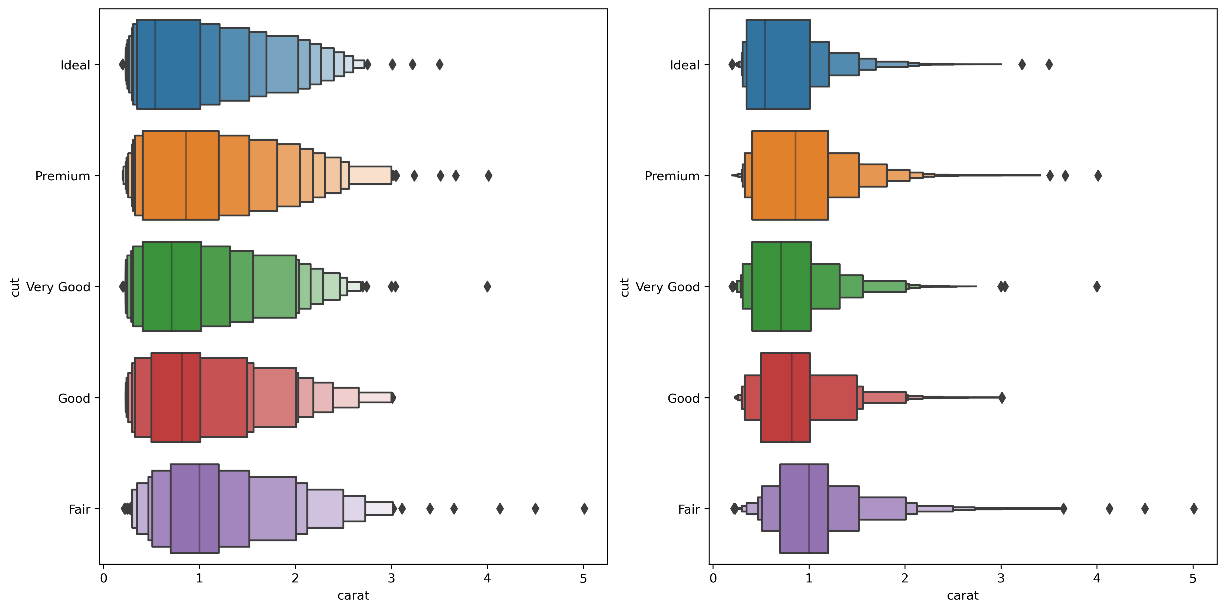
df = sns.load_dataset("diamonds")plt.figure(dpi=300, figsize=(16, 8))# 调整每个箱的宽度plt.subplot(1, 2, 1)sns.boxenplot(data=df, x="carat", y="cut", scale="linear")# 调整箱的个数plt.subplot(1, 2, 2)sns.boxenplot(data=df, x="carat", y="cut", k_depth="trustworthy") |
2.1.3.6 pointplot()
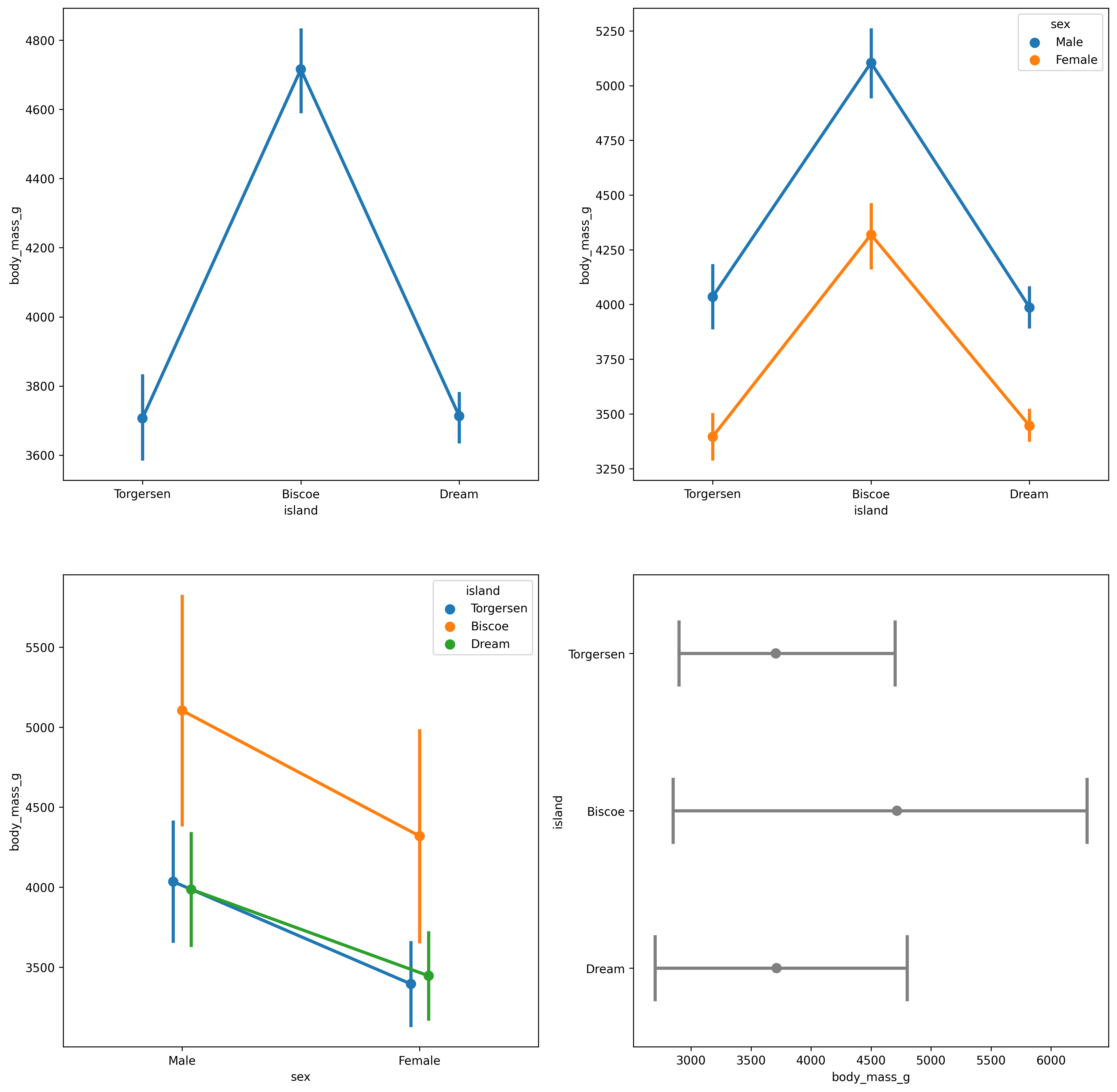
df = sns.load_dataset("penguins")plt.figure(dpi=300, figsize=(16, 16))plt.subplot(2, 2, 1)sns.pointplot(data=df, x="island", y="body_mass_g")plt.subplot(2, 2, 2)sns.pointplot(data=df, x="island", y="body_mass_g", hue="sex")# 使用标准差绘制误差线plt.subplot(2, 2, 3)sns.pointplot(data=df, x="sex", y="body_mass_g", hue="island", dodge=True, errorbar="sd")# 自定义一些图形参数plt.subplot(2, 2, 4)sns.pointplot(data=df, x="body_mass_g", y="island", errorbar=("pi", 100), capsize=.4, join=False, color=".5" ) |
2.1.3.7 barplot()
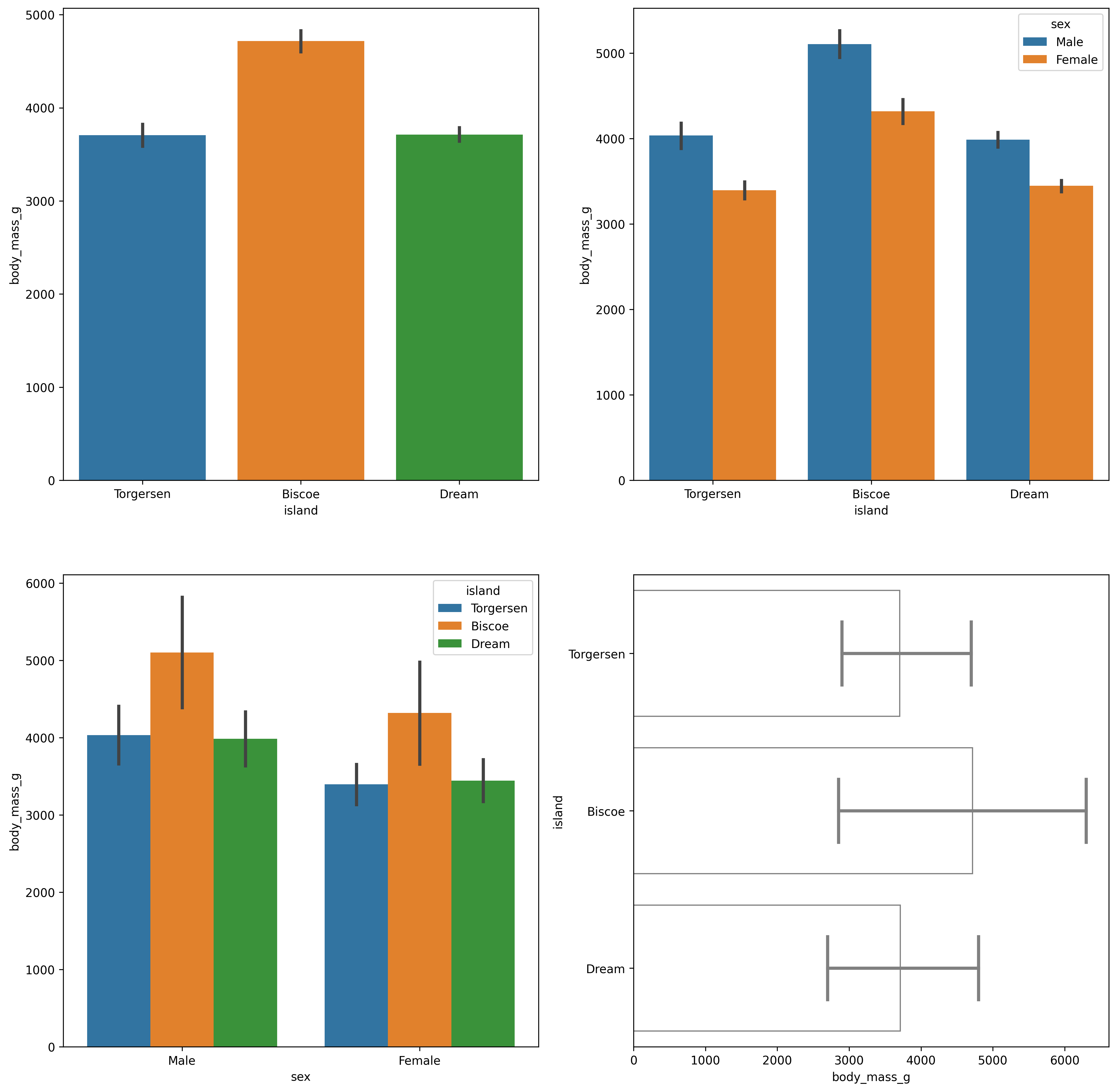
df = sns.load_dataset("penguins")plt.figure(dpi=300, figsize=(16, 16))# 其使用方法和 pointplot 类似plt.subplot(2, 2, 1)sns.barplot(data=df, x="island", y="body_mass_g")plt.subplot(2, 2, 2)sns.barplot(data=df, x="island", y="body_mass_g", hue="sex")plt.subplot(2, 2, 3)sns.barplot(data=df, x="sex", y="body_mass_g", hue="island", dodge=True, errorbar="sd")plt.subplot(2, 2, 4)sns.barplot(data=df, x="body_mass_g", y="island", errorbar=("pi", 100), capsize=.4, edgecolor=".5", errcolor=".5", facecolor=(0, 0, 0, 0) ) |
2.1.3.8 countplot()
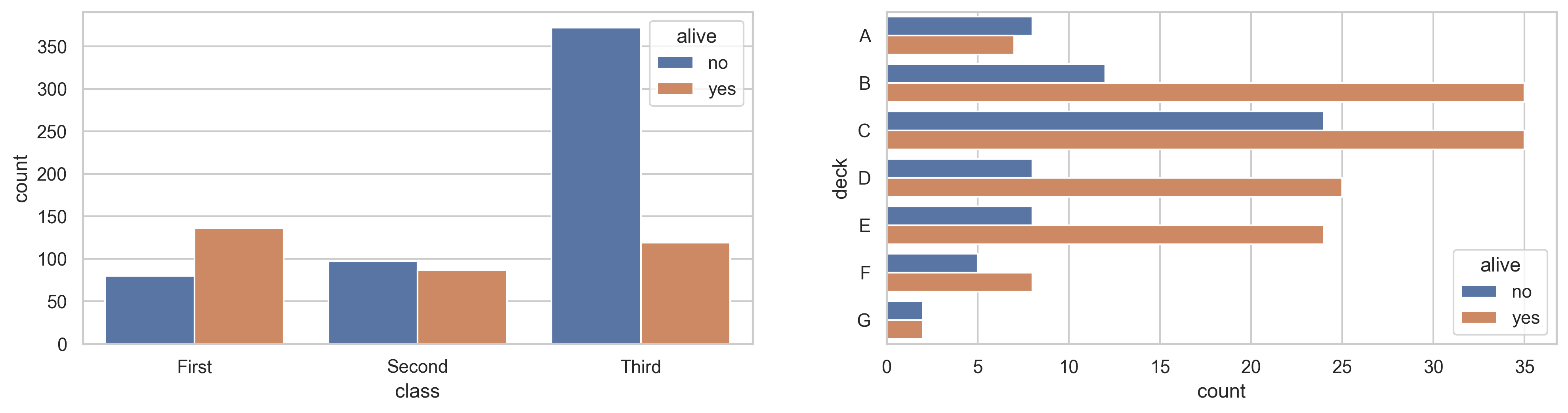
相比之下 countplot() 的使用就更加简单:
sns.set_theme(style="whitegrid")df = sns.load_dataset("titanic")plt.figure(dpi=300, figsize=(16, 8))plt.subplot(2, 2, 1)sns.countplot(data=df, x="class", hue="alive")plt.subplot(2, 2, 2)sns.countplot(data=df, y="deck", hue="alive") |
2.1.4 回归模型分析型
2.1.4.1 lmplot()
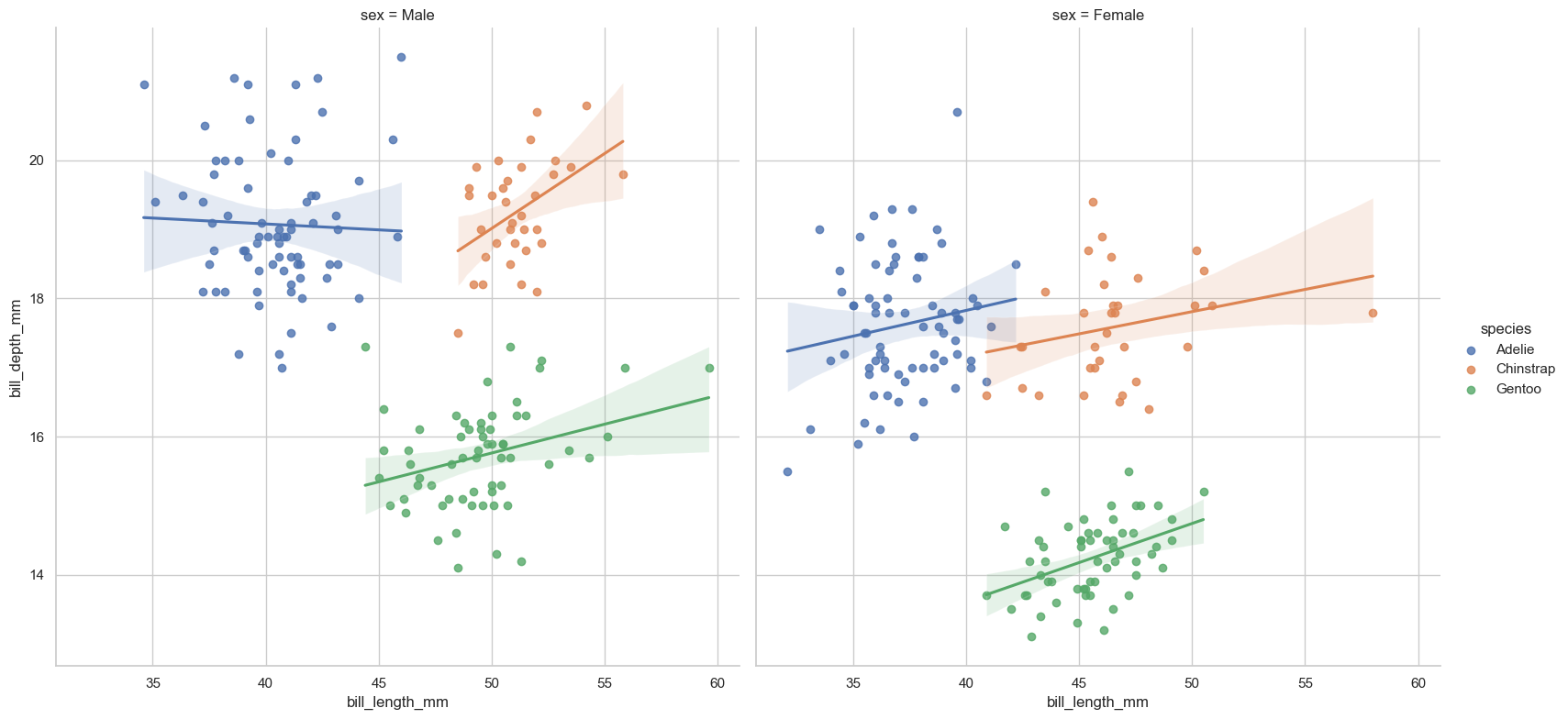
该函数在绘制数据散点的同时对其调用回归模型对其进行拟合,它结合了regplot()和FacetGrid(),从其参数列表也可以看出。
penguins = sns.load_dataset("penguins")sns.lmplot(data=penguins, x="bill_length_mm", y="bill_depth_mm", hue="species") |
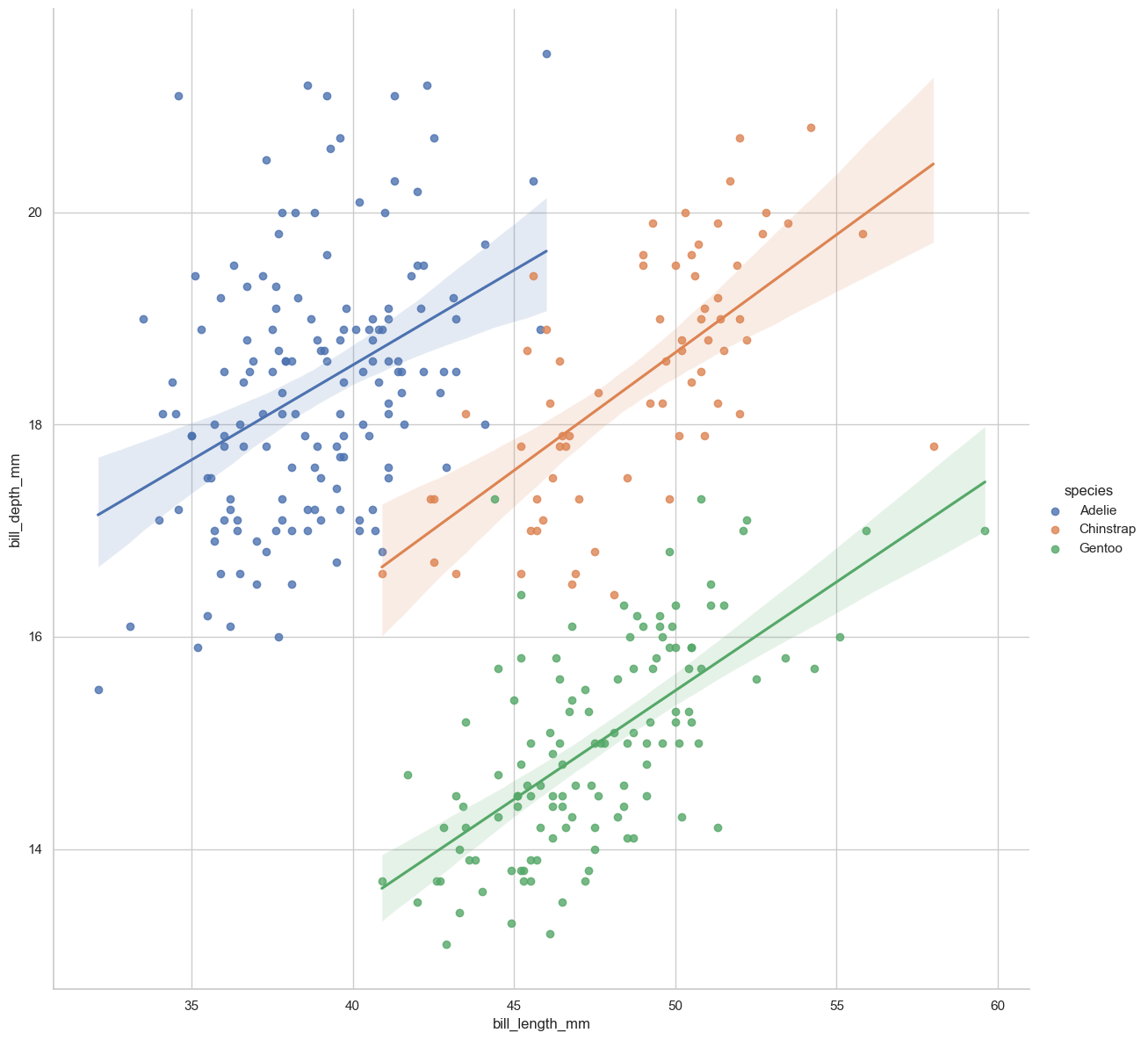
可以绘制多子图同时观察不同类别下的数据拟合情况
sns.lmplot(data=penguins, x="bill_length_mm", y="bill_depth_mm", hue="species", col="sex", height=8) |
2.1.4.2 regplot()
lmplot()以涵盖其全部功能,故不再赘述
2.1.4.3 residplot()
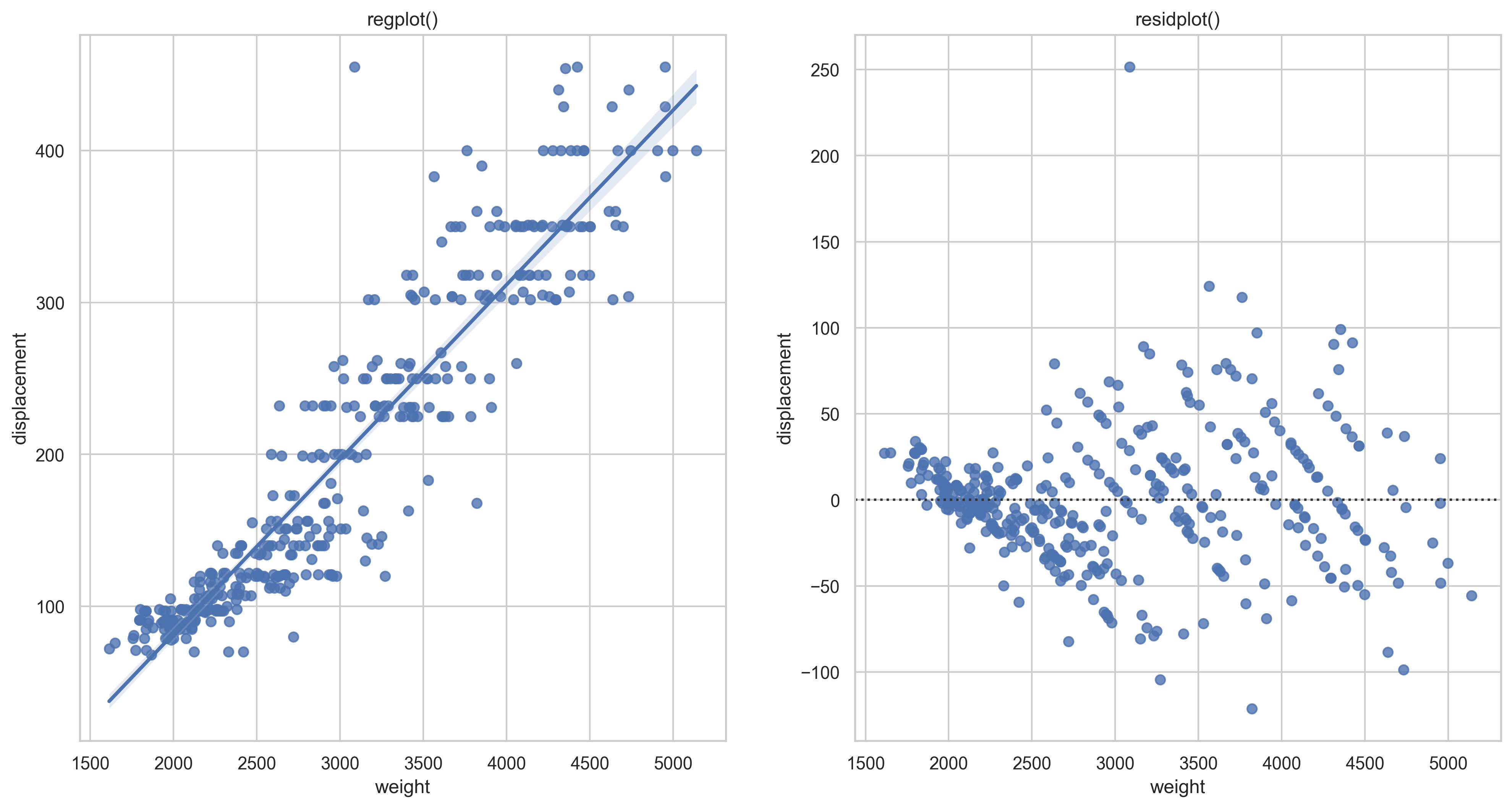
residplot()绘制你和结果的残差。
mpg = sns.load_dataset("mpg")plt.figure(dpi=300, figsize=(16, 8))plt.subplot(1, 2, 1)plt.title("regplot()")sns.regplot(data=mpg, x="weight", y="displacement")plt.subplot(1, 2, 2)plt.title("residplot()")sns.residplot(data=mpg, x="weight", y="displacement", order=2) |
2.2 多子图网格型图
2.2.1 FacetGrid 类
| Methods or Attributes | Type | Functionality |
|---|---|---|
__init__ |
Method | 初始化matplotlib的figure以及FaceGrid对象 |
add_lengnd |
Method | 绘制图例 |
apply |
Method | 将grid传给某个用户自定义函数,然后返回自身 |
dspine |
Method | 去除坐标轴 |
facet_axis |
Method | 返回某一个axis |
facet_data |
Method | 返回含有所有facet的数据和具名indices的生成器 |
map |
Method | 调用某一个绘图函数作用于facet中的数据的一个子集 |
map_dataframe |
Method | 与.map类似 |
pipe |
Method | 将grid传入一个用户自定义函数并返回对应的值 |
refline |
Method | 在每个子图中添加参考线 |
savefig |
Method | 存储绘图结果 |
set |
Method | 设置每个子图Axes的参数 |
set_axis_labels |
Method | 设置子图的两轴标签 |
set_titles |
Method | 设置子图标题 |
set_xlabels / set_ylabels |
Method | 设置子图的x轴或y轴标签 |
set_xticklabels / set_yticklabels |
Method | 设置子图的x轴或y轴刻度标签 |
tick_params |
Method | 设置刻度参数 |
tight_layout |
Method | 调整子图的布局 |
ax |
Attribute | 未设置facet变量时的Axes |
axes |
Attribute | Axes数组 |
axes_dict |
Attribute | 包含Axes的字典 |
figure |
Attribute | 可通过此调整grid背后的mpl.figure.Figure对象 |
legend |
Attribute | 可通过此调整mpl.legend.Legend对象 |
__init__()
示例
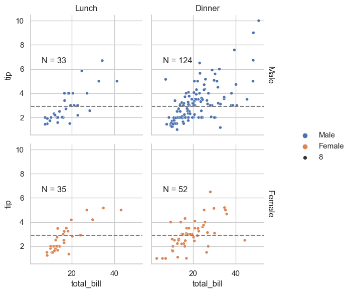
tips = sns.load_dataset("tips")def annotate(data, **kws): n = len(data) ax = plt.gca() ax.text(.1, .6, f"N = {n}", transform=ax.transAxes)g = sns.FacetGrid(data=tips, col="time", row="sex", margin_titles=True)g.set_titles(col_template="{col_name}", row_template="{row_name}")g.map_dataframe(sns.scatterplot, x="total_bill", y="tip", hue="sex")g.map_dataframe(annotate)g.add_legend()g.refline(y=tips["tip"].median()) |
2.2.2 PairGrid 类
| Methods or Attributes | Type | Functionality |
|---|---|---|
__init__ |
Method | 初始化matplotlib的figure以及FaceGrid对象 |
| … | … | … |
map_diag |
Method | 将绘图函数作用于对角线的子图 |
map_lower |
Method | 将函数作用于下三角部分的子图(不包括对角线) |
map_upper |
Method | 将函数作用于上三角部分的子图(不包括对角线) |
map_offdiag |
Method | 将函数作用域除对角线以外的所有子图 |
| … | … | … |
__init__
一些示例
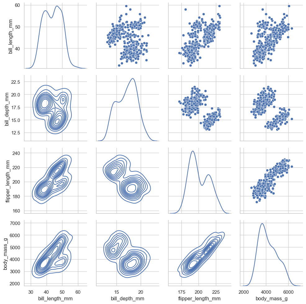
g = sns.PairGrid(penguins, diag_sharey=False)g.map_diag(sns.kdeplot)g.map_lower(sns.kdeplot)g.map_upper(sns.scatterplot) |
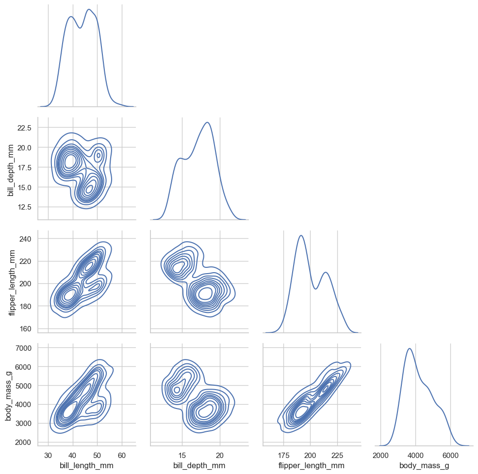
# 仅仅绘制下三角部分g = sns.PairGrid(penguins, diag_sharey=False, corner=True)g.map_diag(sns.kdeplot)g.map_lower(sns.kdeplot) |
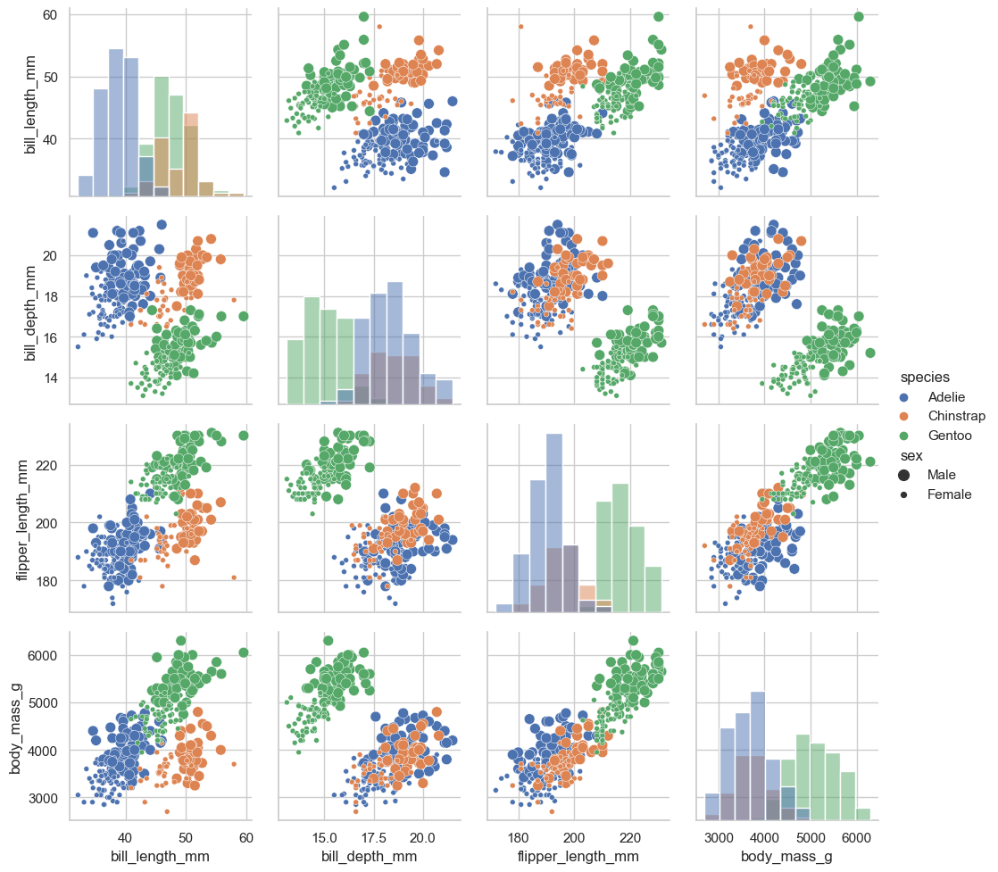
# 使多个函数作用在某些子图中g = sns.PairGrid(penguins, hue="species")g.map_diag(sns.histplot)g.map_offdiag(sns.scatterplot, size=penguins["sex"])g.add_legend(title="", adjust_subtitles=True) |
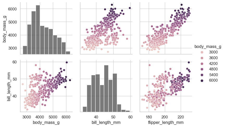
# 设置不同子图的 hue# 并使用 variables 控制传入的变量x_vars = ["body_mass_g", "bill_length_mm", "flipper_length_mm"]y_vars = ["body_mass_g", "bill_length_mm"]g = sns.PairGrid(penguins, hue="body_mass_g", x_vars=x_vars, y_vars=y_vars)g.map_diag(sns.histplot, hue=None, color=".3")g.map_offdiag(sns.scatterplot)g.add_legend() |
2.3 绘图风格、颜色主题和绘图元素缩放比例
2.3.1 绘图风格
2.3.1.1 seaborn.set_theme()
def set_theme(context="notebook", # string or dict; Scaling parameters style="darkgrid", # string or dict; Axes style parameters palette="deep", # string or sequence; Color palette font="sans-serif", # Font family; font_scale=1, # float, optional; color_codes=True, # bool; rc=None # dict or None; matplotlib rc params ):... |
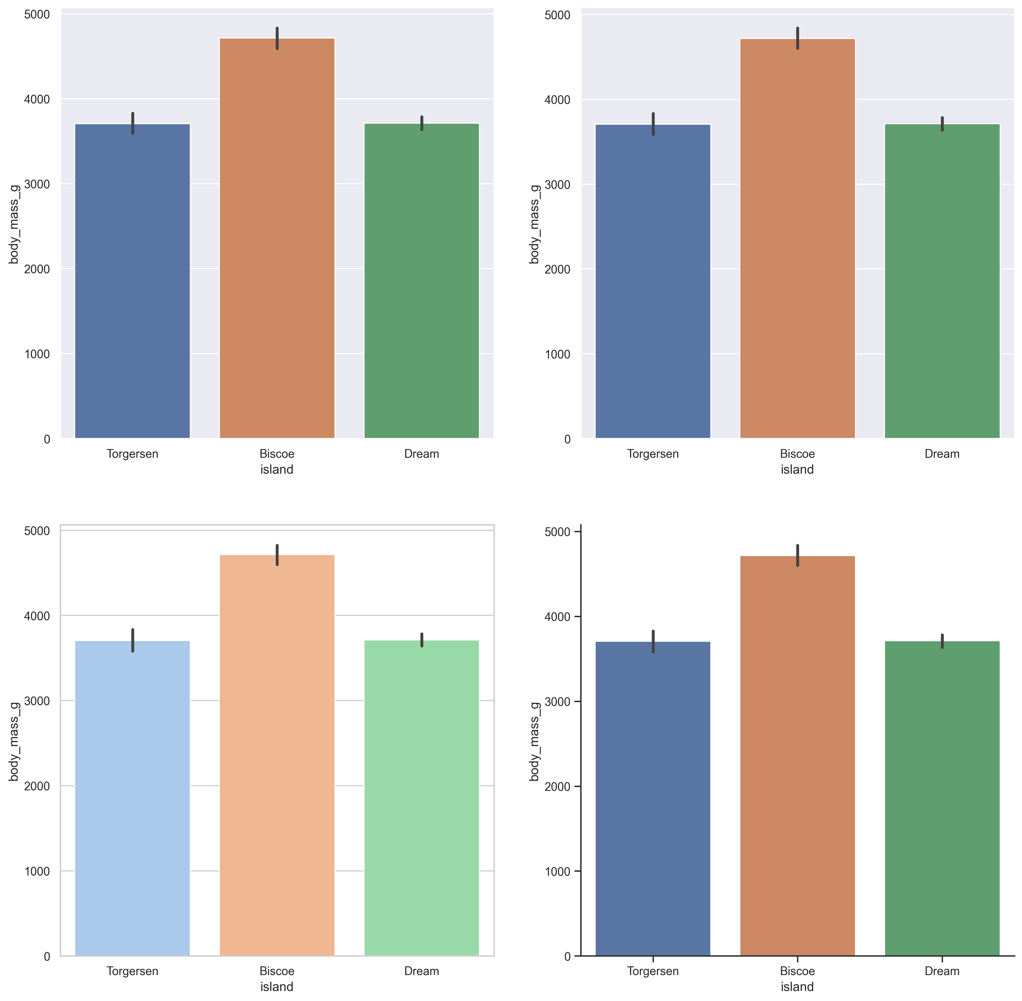
df = sns.load_dataset("penguins")plt.figure(dpi=300, figsize=(16, 16))plt.subplot(2, 2, 1)sns.barplot(data=df, x="island", y="body_mass_g")sns.set_theme()plt.subplot(2, 2, 2)sns.barplot(data=df, x="island", y="body_mass_g")sns.set_theme(style="whitegrid", palette="pastel")plt.subplot(2, 2, 3)sns.barplot(data=df, x="island", y="body_mass_g")custom_params = {"axes.spines.right": False, "axes.spines.top": False}sns.set_theme(style="ticks", rc=custom_params)plt.subplot(2, 2, 4)sns.barplot(data=df, x="island", y="body_mass_g") |
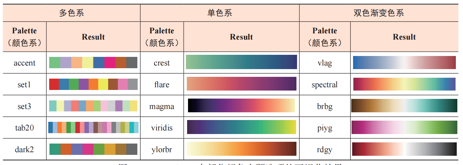
2.3.2 颜色主题
2.3.2.1 应用颜色主题
df = sns.load_dataset("penguins")plt.figure(dpi=300, figsize=(16, 16))plt.subplot(2, 2, 1)sns.barplot(data=df, x="island", y="body_mass_g")sns.set_theme(palette="Accent")plt.subplot(2, 2, 2)sns.barplot(data=df, x="island", y="body_mass_g")sns.set_theme(palette="crest")plt.subplot(2, 2, 3)sns.barplot(data=df, x="island", y="body_mass_g")sns.set_theme(palette="blend:#7AB,#EDA")plt.subplot(2, 2, 4)sns.barplot(data=df, x="island", y="body_mass_g") |
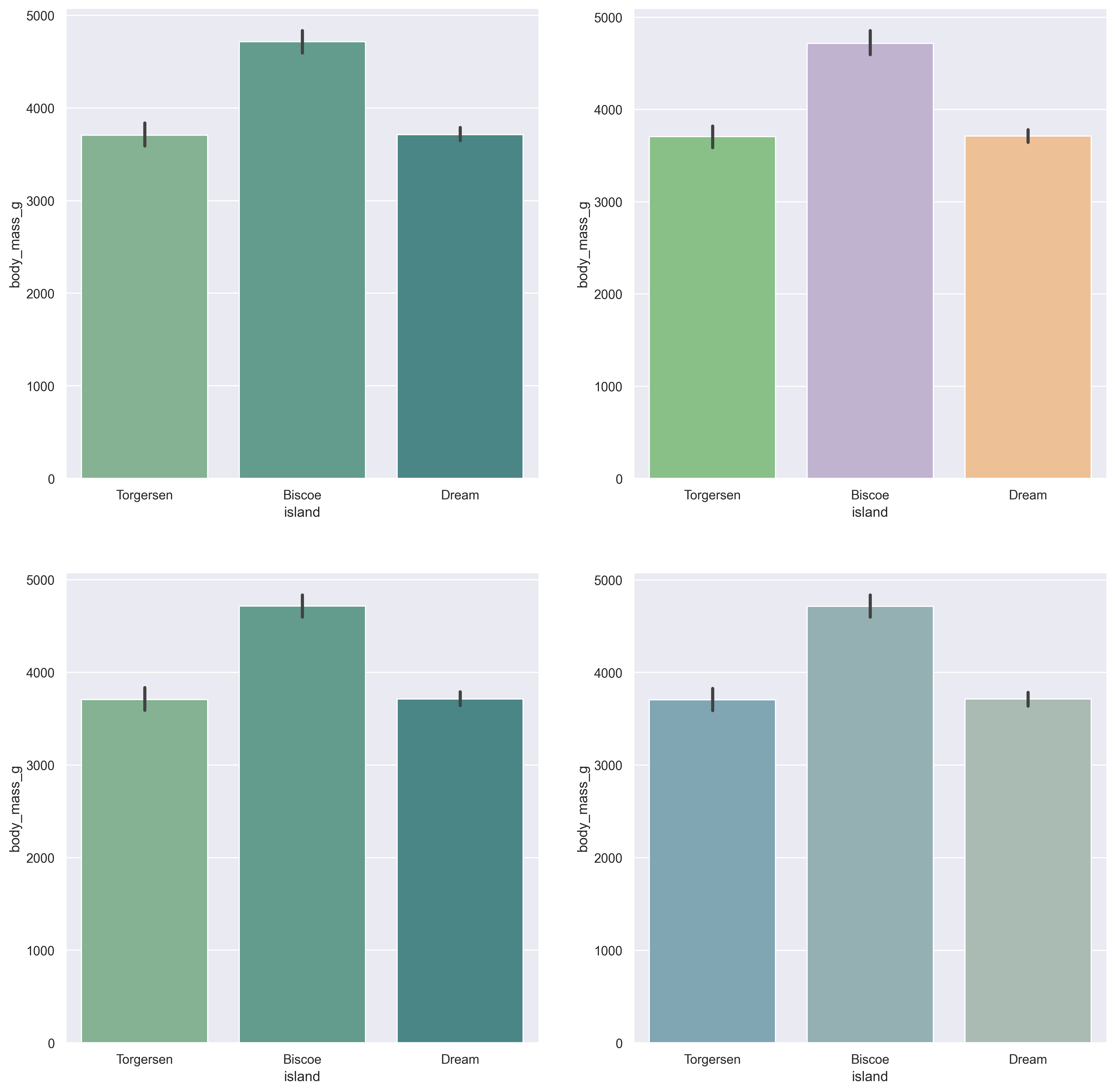
2.3.2.2 使用 color_palette() 自定义色系
sns.color_palette("ch:s=.25,rot=.25") # cubehelix color palettesns.color_palette("light:#5A9") # light sequential gradientsns.color_palette("dark:#5A9_r") # [reversed] dark sequential gradientsns.color_palette("blend:#7AB,#EDA") # blend gradient |




2.3.3 绘图元素缩放比例
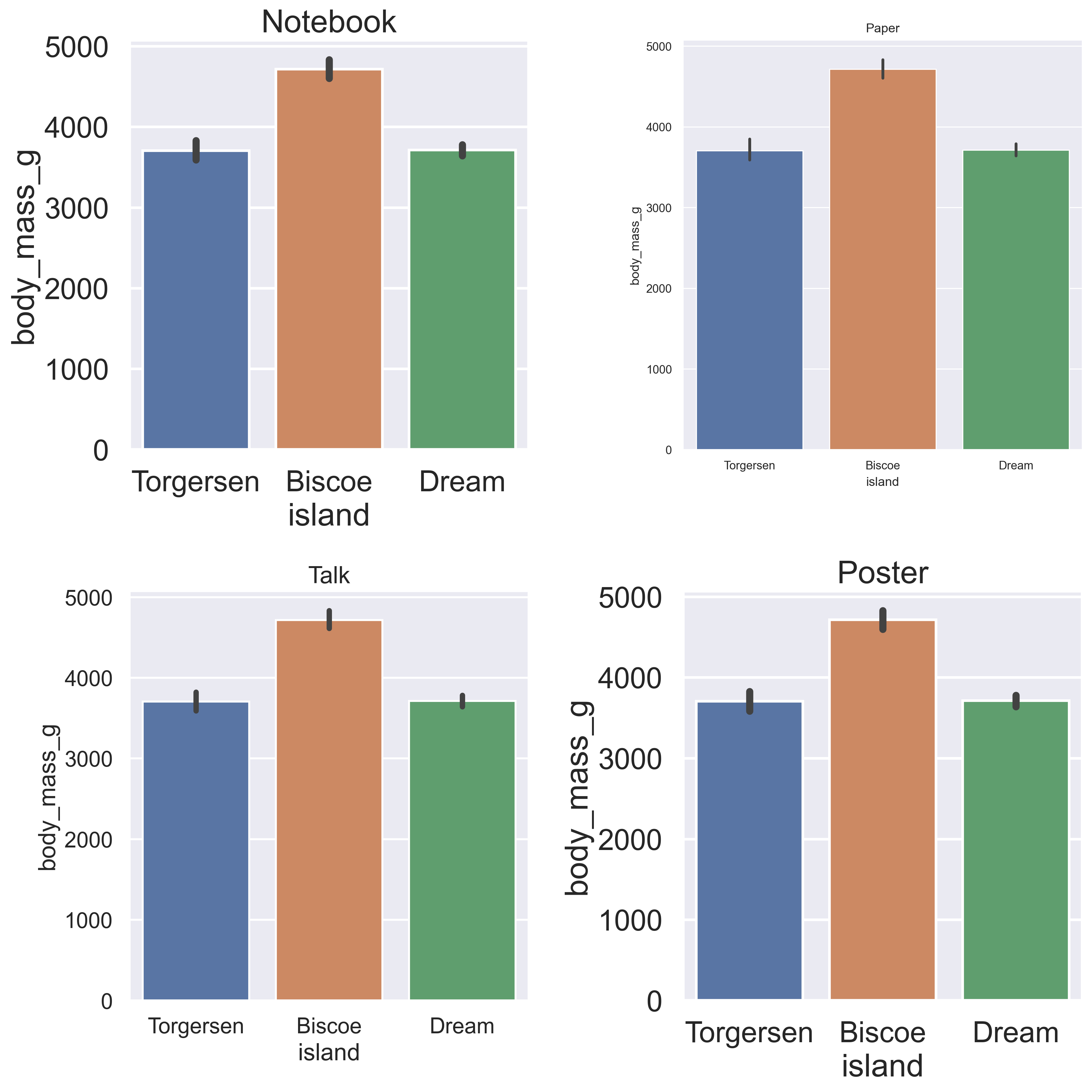
可以通过设置context参数调整绘图元素的相对大小,参数一共接受一下几种:
papernotebooktalkposter
绘图元素的缩放比例依次增大。
df = sns.load_dataset("penguins")plt.figure(dpi=300, figsize=(12, 12))plt.subplot(2, 2, 1)sns.barplot(data=df, x="island", y="body_mass_g")plt.title("Notebook")sns.set_theme(context="paper")plt.subplot(2, 2, 2)sns.barplot(data=df, x="island", y="body_mass_g")plt.title("Paper")sns.set_theme(context="talk")plt.subplot(2, 2, 3)sns.barplot(data=df, x="island", y="body_mass_g")plt.title("Talk")sns.set_theme(context="poster")plt.subplot(2, 2, 4)sns.barplot(data=df, x="island", y="body_mass_g")plt.title("Poster")plt.tight_layout() |