一篇存货

image

2 Fully Hyperbolic Convolutional Neural Networks for Computer Vision

https://openreview.net/forum?id=ekz1hN5QNh

一些问题

  1. Discuss the motivation behind using the Lorentz model instead of the Poincaré ball in this paper. What benefits does it offer? 庞加莱球模型接近边界时的距离函数是无界的,不利于计算((Bdeir et al., 2024, p. 2) (pdf))| 洛伦兹模型中的距离、度量、平移等具有形式较好的解析解、经过零点的测地线到其切空间的投影均为直线、相同维数不同曲率的双曲空间共用一个零点 分母为零,x=y时 cosh(1) cosh(10)
  2. The paper introduces Lorentzian batch normalization. Describe how it generalizes traditional batch normalization for hyperbolic space. 一般的BN层包括减去 μ 和线性放缩两步。而Frechet平均没有解析解,会拖慢模型训练进度。文中提出使用平方双曲距离的centroid作为Frechet平均的一个近似。然后利用零点处测地线投影为直线的性质将双曲空间的点投影至centroid处的切空间后平移至零点切空间,在此进行放缩之后再移回去((Bdeir et al., 2024, p. 5) (pdf))
  3. What is the Lorentzian centroid, and why is it used in batch normalization? Lorentzian centroid以下优化问题的解析解 minμ∈LKn∑i=1mνidL2(xi,μ) 。通过最小化至各点平方双曲距离之和作为Frechet平均的一个近似,而后者难以在短时间内通过迭代得到足够好的逼近。
  4. Derive and explain the formula for the distance between a point and a hyperplane in the Lorentz model as presented in the paper. 附录写了,双曲空间中的点可以关于超平面获取其镜像。该点和镜像的测地线段等于该点至超平面距离的两倍。
  5. Review the implementation of the Lorentz convolutional layer in the code repository. How does it handle feature maps and kernel operations? 将每个要做卷积的kernel提出来,然后reshape好,对所有的patches做lorentz fully connected运算
  6. How is parallel transport used in the code, and why is it critical for operations in hyperbolic space? 用于BN层和Wrapped Normal分布(VAE里面用的,但我还没看)。 对于双曲空间中非零点的切空间,其测地线在切空间上的投影是曲线,不好控制。
  7. Examine how the paper implements residual connections in the Lorentz model. What challenges arise, and how are they addressed? 当stride不为1或输出维数不为预测维数时会产生形状不对齐的情况,作者采用的方法是使用1x1卷积带上stride参数进行调整
  8. If you were to improve the HCNN framework, what additional components or optimizations would you suggest? 考虑Attention?(类似第一篇文章)优化方面考虑在除了pytorch模块运行之外的双曲空间上的若干操作,如指数对数映射,parallel transport是否消耗太多时间,是否可以使用差一些精度的近似来提高速度

Hyperbolic Geometry

The n -dimensional hyperbolic space HKn is a Riemannian manifold (Mn,gxK) with constant negative curvature K<0 , where Mn represents the manifold while gxK represents the Riemann metric.

Poincaré ball The n -dimensinoal Poincaré ball BKn=(Bn,gxK) is defined by Bn={x∈Rn|−K∥x∥2<1} and the Riemann metric gxK=(λxK)2In , in which λxK=21+K∥x∥2 . It describes an open ball with radius −1K .

Lorentz Model The n -dimensional Lorentz model LKn=(Ln,gxK) models hyperbolic geometry on the upper sheet of a two theeted hyperboloid Ln , with origin 0¯=[−1K,0,…,0] and embedded in (n+1) -dimensinoal Minkowski space. The Riemann metric gxK=diag(−1,1,…,1) and the manifold is defined as

Ln:={x∈Rn+1|⟨x,x⟩L=1K,xt>0},

with the Lorentzian inner product

⟨x,y⟩L:=−xtyt+xs⊤yt=x⊤diag(−1,1,…,1)y.

We call the first component the time component xt and the remaining part space component xs s.t. x=[xt,xs]⊤∈LKn and xt=∥xs∥2−1K
image

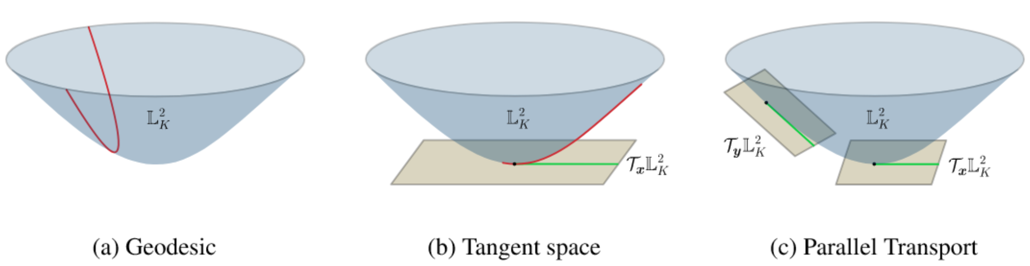
Distance on Lorentz Model The shortest path on the model is inherited from Minkowski space. Let x,y∈LKn , the length of the connecting geodestic is given by

dL(x,y)=1−1/Kcosh−1⁡(K⟨x,y⟩L),dL2(x,y)=∥x−y∥L2=2K−2⟨x,y⟩L.

When calculating distance to origin 0¯ , the terms can be simplified to

dL(x,0¯)=∥log0¯K⁡(x)∥,dL2(x,0¯)=2K(1+−Kxt).

Tangent Space on Lorentz Model The space around each point x on a differentiable manifold M can be linearly approximated by the tangent space TxM . Let x∈LKn , the tangent space at point x can be experssed as

TxLKn:={y∈Rn+1|⟨y,x⟩L=0}

Exponential and Logarithmic Maps on Lorentz Model Exponential and logarithmic maps between manifold M and tangent space TxM with x∈M .

expxK⁡(z)=cosh⁡(α)x+sinh⁡(α)zα,with α=−K∥z∥L,∥z∥L=⟨z,z⟩LlogxK⁡(y)=cosh−1⁡(β)β2−1⋅(y−βx),with β=K⟨x,y⟩L

When dealing with tangent space at origin 0¯ , the exponential map simplifies to

exp0¯K⁡(z)=1−K[cosh⁡(−K∥z∥),sinh⁡(−K∥z∥)z∥z∥]

Fully Hyperbolic CNN

Hyperbolic Feature Maps Adding Lotentz model's time component as additional channel dimension, which difines a hyperbolic feature mao as an ordered set of n -dimensional hyperbolic vectors. #HELP

Lorentz Fully-connected Layer Let x∈LKn and W∈Rm×(n+1) and v∈Rn+1 are weight params. Then the transformation matrix is

f(x)(M)=fx([v⊤W])=[∥Wx∥2−1/Kv⊤xv⊤W].

Adding other compo nents including normalization, the Lorentz fully connected layer becomes

y=[∥ϕ(Wx,v)∥2−1/Kϕ(Wx,v)],

in which

ϕ(Wx,v)=λσ(v⊤x+b′)Wψ(x)+b∥Wψ(x)+b∥.

If normalization is removed, the Lorentz fully-connected layer becomes

y=LFC(x)=[∥ψ(Wx+b)∥2−1/Kψ(Wx+b)],

Hyperbolic Direct Concat Given a set of hyperbolic points {xi∈LKn}i=1N , the Lorentz concatenation is given by

y=HCat({xi}i=1N)=[∑i=1Nxi,t2+N−1K,x1,s⊤,…,xN,s⊤]⊤∈LKnN⊂RnN+1

Lorentz Convolutional Layer Convolution layer is a matrix multiplication between a linearized kernel and a concatenation of the values in its receptive field. Then we generalize this definition by replacing Euclidean operators with hyperbolic counterparts. Given hyperbolic input feature map x={xh,w∈Lkn}h,w=1H,W as an ordered set of n -dimensional hyperbolic feature vectors, each describing image pixels. The kernel is K∈Rm×n×H~×W~ with respective field {xh′+δh~,w′+δw~∈LKn}h~,w~=1H~,W~ in which (h′,w′) denotes starting position and δ denotes stride. (Why stride ??)

The Lorentz convolutional layer is

yh,w=LFC(HCat({xh′+δh~,w′+δw~∈LKn}h~,w~H~,W~))

in which HCat denotes the concatenation of hyperbolic vectors and LFC denotes a Lorentz fully connected layer.

Parallel Tramsport on Lorentz Model The parallel transport operation PTx→yK(v) maps a vector v∈TxM from the tangent space of x∈M to the tangent space of y∈M . It preserves the local geometry around the reference point by moving the points along the geodesic connecting x and y . The formula for the Lorentz model is given by

PTx→yK(v)=v−⟨logxK⁡(y),v⟩LdL(x,y)(logxK⁡(y)+logyK⁡(x))=v+⟨y,v⟩L1−K−⟨x,y⟩L(x+y).

Lorentzian Centroid The weighted centroid with respect to the squared Lorentzian distance, which solves minμ∈LKn∑i=1mνidL2(xi,μ) with xi∈LKn and νi⩾0,∑i=1m>0 , is given by

μ=∑i=1mνixi−K|‖∑i=1mνixi‖L|.

Lorentz Batch Normalization We generalize batch normalization to the Lorentz model using the Lorentzian centroid and the parallel transport operation for re-centering, and the Fréchet variance and straight geodesics at the origin’s tangent space for re-scaling.

Re-centering Usually Fréchet mean is used, which minimizes the expected distance between set of points in a metric space. However it requires iterative computation, which significantly slows down training process. We use closed form of centeroid w.r.t. Lorentzian distance.

In batch norm, weights are equally assigned, i.e. νi=1m . Then we shift the features from batch mean μB to parametrized mean β (learnable parameters) by applying parallel transform PTμB→βK(x) . Note that parallel transport does not change the variance. During training the param is updated iteratively with weight 1−η and η .

Re-scaling We rely on Fréchet variance defined as expected squared Lorentzian distance between points and mean, given by σ2=1m∑i=1mdL2(xi,μ) . In order to rescale the batch, features should be moved along the geodestic connecting them and centeroid.Though geodestics intersecting at the centeroid is infeasible to compute, the ones intersecting at the origin is simple. Thus we consider first parallely transport features to the origin, scale them and then transport them back to original centeroid:

LBN(x)=expβK⁡[PT0¯→βK(γ⋅PTμB→0¯K(logμBK⁡(x))σB2+ϵ)].

Lorentz MLR Classifier

Hyperplane in the Lorentz Model

The hyperplane in the Lorentz model is defined by a geodestic that results from the intersection of an n -dimensional hyperplaine with the hyperboloid in the ambient space Rn+1 . Specifically, for p∈LKn and w∈LKn , the hyperplane passing through p and perpendicular to w is given by

Hw,p={x∈LKn|⟨w,x⟩L=0}.

As w is parametrized by vector z¯ , which can be parallel transported to p :

z¯=[0,az∥z∥]∈T0¯LKn,w:=PT0¯→pK(z¯)=[sinh⁡(−Ka)∥z∥,cosh⁡(−Ka)z],

in which z∈Rn and a∈R . We can rewrite the hyperplane as

H~z,a={x∈Lkn|cosh⁡(−Ka)⟨z,xs⟩−sinh⁡(−Ka)∥z∥xt=0},

where a and z represents the distance and orientation to the origin respectively.

Theorem. Minimum Hyperbolic Distance

Given a∈R and z∈Rn , the minimum hyperbolic distance from a point x∈Lkn to the hyperplane H~z,a is given by

dL(x,H~z,a)=1−K|sinh−1⁡[−Kcosh⁡(−Ka)⟨z,xs⟩−sinh⁡(−Ka)∥z∥xt∥cosh⁡(−Ka)z∥2−(sinh⁡(−Ka)∥z∥)2]|.

Proof. Note that the distance from point x∈LKn to hyperplane Hw,p equals half of the distance between the point and its reflection in the hyperplane yw :

\begin{aligned} \mathbf{y}_{\mathbf{w} } &= \mathbf{x} + \frac{2\left\langle \mathbf{w}, \mathbf{x} \right\rangle_{\mathcal{L} }\mathbf{w} }{\left\langle \mathbf{w}, \mathbf{w} \right\rangle_{\mathcal{L} } }, \tag{a}\\ d_{\mathcal{L} }(\mathbf{x}, H_{\mathbf{w}, \mathbf{p} }) &= \frac{1}{2} d_{\mathcal{L} }(\mathbf{x}, \mathbf{y}_{\mathbf{w} }).\tag{b} \end{aligned}

where w is perpendicular to the hyperplane. Inserting (a) into (b) and we have

dL(x,Hw,p)=12−Kcosh−1⁡(K⟨x,yw⟩L)=12−Kcosh−1⁡(K⟨x,x+2⟨w,x⟩Lw⟨w,w⟩L⟩)Injecting (a)=12−Kcosh−1⁡(K⟨x,x⟩+2⟨x,⟨w,x⟩Lw⟨w,w⟩L⟩)Lineararity=12−Kcosh−1⁡[1+2(−K⟨w,x⟩L⟨w,w⟩L)2]Hyperbolic Inner Product=1−K|sinh−1⁡(−K)⟨w,x⟩L∥w∥L|

Finally we insert reparametrization of w into the above term and gives the final distance formula.

Theorem. Output Logit of the Lorentz MLR Given parameters ac∈R and zc∈Rn , the Lorentz MLR's output logit corresponding to class c and input x∈LKn is given by

vzc,ac(x)=1−Ksign(α)β|sinh−1⁡(−Kαβ)|,α=cosh⁡(−Ka)⟨z,xs⟩−sinh⁡(−Ka),β=∥cosh⁡(−Ka)z∥2−(sinh⁡(−Ka)∥z∥)2

Lorentz Residual Connection and Activation we add the vector’s space components and concatenate a corresponding time component.

Non-linear Activation
We propose a simpler operation for the Lorentz model by applying the activation function to the space component and concatenating a time component.

y=[∥ReLU(xs)∥2−1/KReLU(xs)]