绘图工具与实例:matplotlib
1 matplotlib
1.1 图形元素
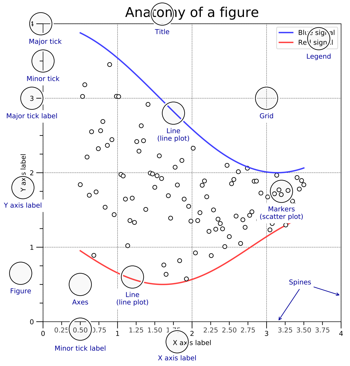
主要图形元素
- 画布(Figure)
- 坐标图形(Axes)
- 轴(Axis)
- 艺术对象(Artist)
图层属性
- 图名(Title)
- 刻度(Tick)
- 刻度标签(Tick Label)
- 轴标签(Axis Label)
- 轴脊(Spine)
- 图例(Legend)
- 网格(Grid)
- 线(Line)
- 数据标记(Marker)
1.2 图层顺序
matplotlib采用面向对象的绘图方式,设置绘图函数中的zorder来指定不同图层。
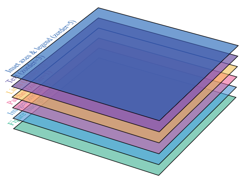
| Artist | zorder |
|---|---|
| Images(AxesImage,FigureImage,BboxImage) |
|
| Patch / PatchCollection |
|
| Line2D / LineCollection |
|
| Text |
|
| Inset axes / Legend |
|
1.3 轴比例和刻度
轴对象可以控制轴比例(Axis Scale)、刻度位置(Tick Locator)和刻度格式(Tick Formatter)
1.3.1 轴比例
matplotlib内实现了线性、对数等轴比例方式,也可以自定义函数比例。
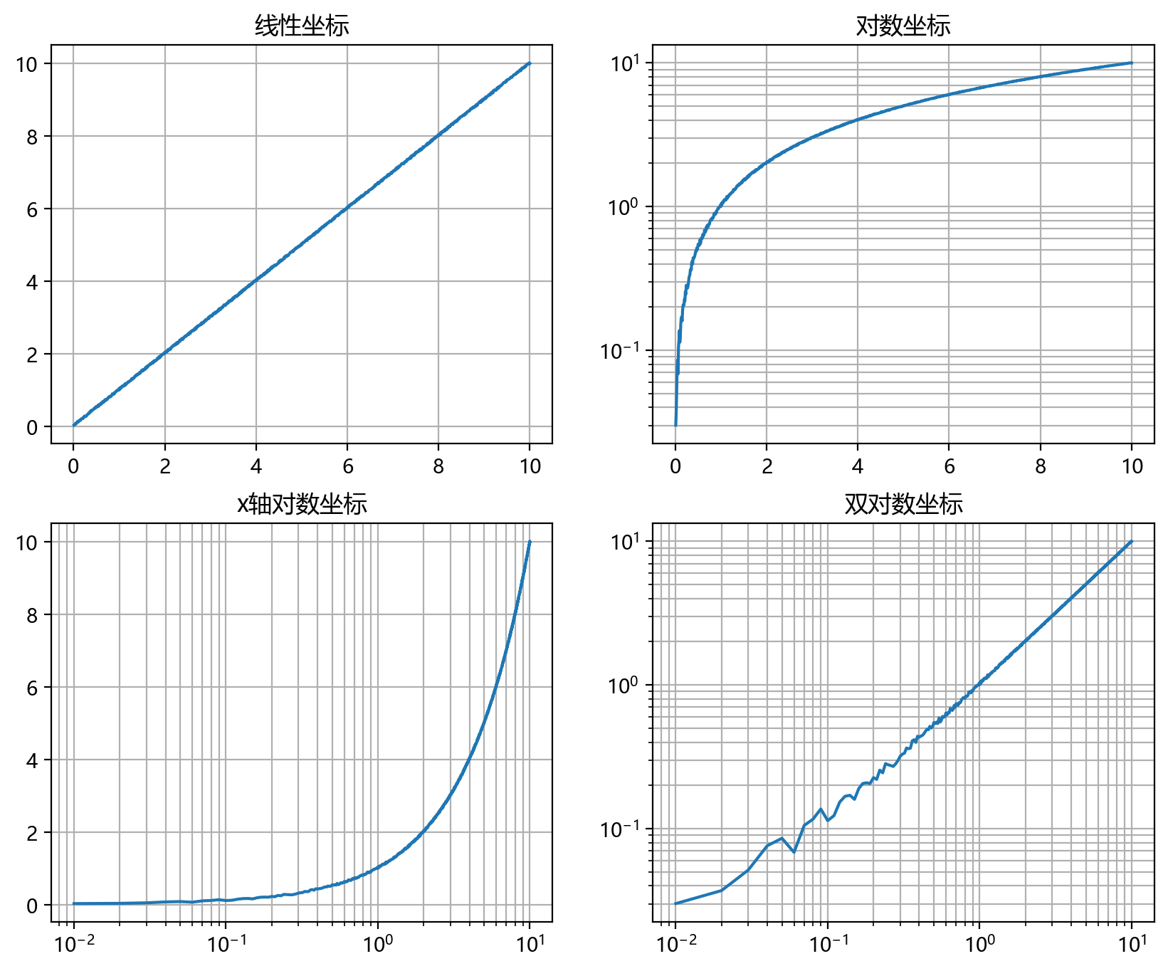
# 导入相关的包import numpy as npimport matplotlib.pyplot as pltimport matplotlib# 初始化设置plt.rcParams['font.family'] = "Microsoft YaHei" # 解决中文显示问题plt.rcParams['axes.unicode_minus'] = False # 解决unicode负号显示问题# 绘图设置 plt.figure(figsize=(10, 8), dpi=200) # 设置画布# 绘制多子图plt.subplot(221) # 两行两列中的第一个子图plt.plot(v, y) # 绘制折线图plt.title("线性坐标") # 设置子图标题plt.grid() # 设置网格ax = plt.subplot(222)plt.title("对数坐标")ax.set_yscale("log"); # 设置 y 轴标度plt.plot(v, y)plt.grid()ax = plt.subplot(223)ax.set_xscale("log");ax.set_yscale("log");plt.title("双对数坐标")plt.plot(v, y)plt.grid()ax = plt.subplot(224)plt.title("对称对数坐标")ax.set_yscale("symlog")plt.plot(v, y)plt.grid()plt.show() |
1.3.2 刻度位置和刻度格式
| 刻度位置与格式 | 解释 | 图示 |
|---|---|---|
NullLocator() |
空轴 |  |
MultipleLocator(0.5) |
包含主刻度和次刻度 |  |
FixedLocator([0, 0.1, 0.3, 0.5, 0.9]) |
选定刻度 |  |
LinearLocator(numticks) |
线性刻度 |  |
IndexLocator(base=0.5, offset=0.3) |
序列刻度 | |
AutoLocator() |
自动刻度 |  |
MaxNLocator() |
设置最大值的刻度 |  |
LogLocator(base=10, ticks=15) |
对数刻度 |  |
NullFormatter() |
无格式化字符串 |  |
StrMethodFormatter("{x:.3f}") |
使用格式化的刻度字符串 |  |
FuncFormatter("{:.3f}".format) |
使用格式化函数格式化刻度字符串 |  |
FixedFormatter(['A'...'K']) |
确定模式的刻度字符串 |  |
ScalarFormatter() |
标量格式化刻度字符串 |  |
FormatStrFormatter("#%d") |
格式化刻度字符串 |  |
PercentFormatter(xmax=8) |
百分比格式化刻度字符串 |  |
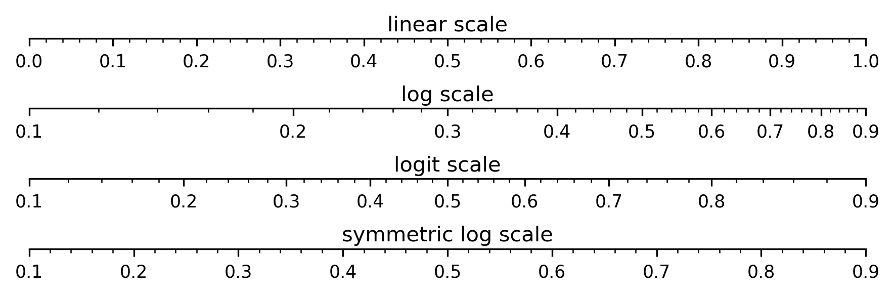
fig = plt.figure(figsize=(6, 2), dpi=300)# 隐藏上、左、右三个方向的边框def unvisible_spines(ax:plt.Axes) -> None: ax.spines["right"].set_visible(False) ax.spines["left"].set_visible(False) ax.spines["top"].set_visible(False)def set_ticks(ax:plt.Axes, maj_loc=0.10, ) -> None: """设置x坐标轴的标度格式, 从上至下依次为 * 主刻度间隔 (0.1) * 主刻度格式 (一位浮点数) * 副刻度间隔 (0.02) * 副刻度格式 (不显示) """ ax.xaxis.set_major_locator(ticker.MultipleLocator(0.10)) ax.xaxis.set_major_formatter(ticker.FormatStrFormatter("%.1f")) ax.xaxis.set_minor_locator(ticker.MultipleLocator(0.02)) ax.xaxis.set_minor_formatter(plt.NullFormatter())# kwargs字典,设置子图x轴和y轴的范围subplot_args = {"xlim":[0, 1], "ylim":[0, 1]}# 线性标度# ------------------------------------------------ax = plt.subplot(4, 1, 1, **subplot_args)ax.set_yticks([])ax.text(0.5, 0.2, "linear scale", transform=ax.transAxes, horizontalalignment="center", verticalalignment="bottom", )unvisible_spines(ax)set_ticks(ax)subplot_args = {"xlim":[0.1, 0.9], "ylim":[0, 1]}# 对数标度# ------------------------------------------------ax = plt.subplot(4, 1, 2, **subplot_args)ax.set_yticks([])ax.text(0.5, 0.2, "log scale", transform=ax.transAxes, horizontalalignment="center", verticalalignment="bottom", )ax.set_xscale("log")unvisible_spines(ax)set_ticks(ax)# Logit 标度# ------------------------------------------------ax = plt.subplot(4, 1, 3, **subplot_args)ax.set_yticks([])ax.text(0.5, 0.2, "logit scale", transform=ax.transAxes, horizontalalignment="center", verticalalignment="bottom", )ax.set_xscale("logit")unvisible_spines(ax)set_ticks(ax)# symlog 标度# ------------------------------------------------ax = plt.subplot(4, 1, 4, **subplot_args)ax.set_yticks([])ax.text(0.5, 0.2, "symmetric log scale", transform=ax.transAxes, horizontalalignment="center", verticalalignment="bottom", )ax.set_xscale("symlog")unvisible_spines(ax)set_ticks(ax)plt.tight_layout() |
1.4 坐标系
常用的坐标系有直角坐标系(Rectangular Coordinate System)、极坐标系(Polar Coordinate System)、地理坐标系(Geographic Coordinate System)
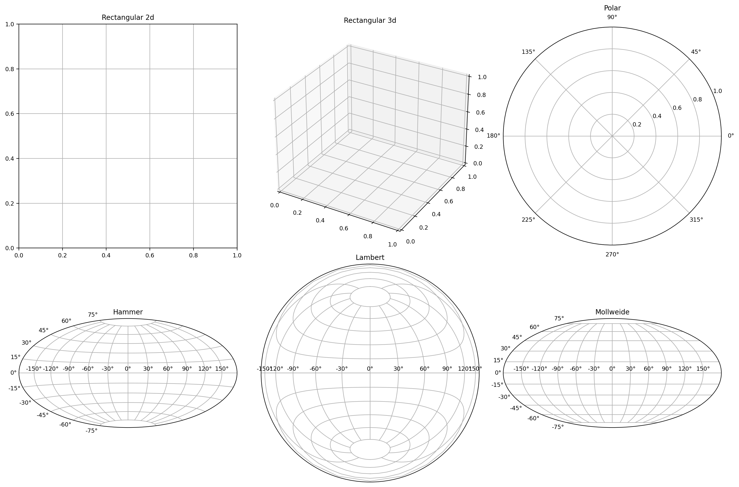
plt.figure(figsize=(15, 10), dpi=200)plt.subplot(2, 3, 1)plt.title("Rectangular 2d")plt.grid()plt.subplot(2, 3, 2, projection="3d")plt.title("Rectangular 3d")plt.grid()plt.subplot(2, 3, 3, projection="polar")plt.title("Polar")plt.subplot(2, 3, 4, projection="hammer")plt.title("Hammer")plt.grid()plt.subplot(2, 3, 5, projection="lambert")plt.title("Lambert")plt.grid()plt.subplot(2, 3, 6, projection="mollweide")plt.title("Mollweide")plt.grid()plt.tight_layout() |
1.5 多子图绘制
由于前文已经大量使用子图的绘制,在此着重讨论一些较为复杂的之图绘制方法
1.5.1 axes()
axes()函数返回可使用在当前画布中的坐标图形对象,其调用形式如下:
plt.axes()plt.axes(rect, projection=None, polar=False, **kwargs)plt.axes(ax) |
我们可以使用axes()的返回对象规定热力图的颜色映射参照colobar()的行为,如下图所示。axes()内可接受四元组参数(视版本而定,也可能是四元列表参数)rect,其中的四个分量分别表示矩形对象的位置(左右和上下)以及矩形对象的形状(宽度和高度)
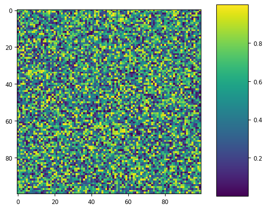
import numpy as npimport matplotlib.pyplot as pltnp.random.seed(19680801)plt.imshow(np.random.random((100, 100)))cax = plt.axes((0.85, 0.10, 0.1, 0.8))plt.colorbar(cax=cax) |
1.5.2 subplot2grid()
该函数可以实现不规则(不完全对齐)的子图绘制,其调用格式如下
subplot2grid(shape, loc, rowspan=1, colspan=1, fig=None, **kwargs) |
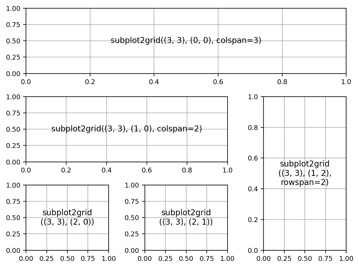
import matplotlib.pyplot as pltdef add_text_center(ax:plt.Axes, text:str) -> None: ax.text(.5, .5, text, horizontalalignment='center', verticalalignment='center',)fig = plt.figure(dpi=200)# 表示该子图形状为 (3, 3),锚点(左上角)位置是 (0, 0),总共占三行ax1 = plt.subplot2grid((3, 3), (0, 0), colspan=3)ax1.grid()add_text_center(ax1, "subplot2grid((3, 3), (0, 0), colspan=3)")ax2 = plt.subplot2grid((3, 3), (1, 0), colspan=2)ax2.grid()add_text_center(ax2, "subplot2grid((3, 3), (1, 0), colspan=2)")ax3 = plt.subplot2grid((3, 3), (1, 2), rowspan=2)ax3.grid()add_text_center(ax3, "subplot2grid\n((3, 3), (1, 2),\nrowspan=2)")ax4 = plt.subplot2grid((3, 3), (2, 0))ax4.grid()add_text_center(ax4, "subplot2grid\n((3, 3), (2, 0))")ax5 = plt.subplot2grid((3, 3), (2, 1))ax5.grid()add_text_center(ax5, "subplot2grid\n((3, 3), (2, 1))")plt.tight_layout() |
1.5.3 gridspec.GridSpec()
gridspec.GridSpec()函数用于指定放置子图网格的几何形状,该类的__init__()函数签名如下
def __init__(nrows, ncols, figure=None, left=None, bottom=None, right=None, top=None, wspace=None, hspace=None, ... ): ... |
其中
nrows和ncols分别设置网格的行数和列数left,bottom,right和top设定网格在整个画布中的位置wspace和hspace分别控制子图之间的水平和垂直间隔
我们也可以使用该函数实现和上面一样的多子图结构,由于和ndarray的数组索引方式相似,在使用时会比较方便。
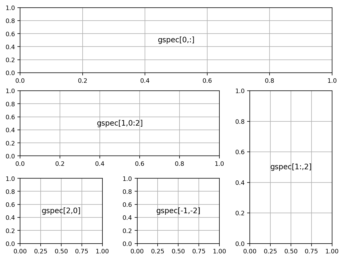
import matplotlib.pyplot as pltimport matplotlib.gridspec as gridspecfig = plt.figure(dpi=200, constrained_layout=True)gspec = gridspec.GridSpec(ncols=3, nrows=3, figure=fig)ax1=plt.subplot(gspec[0,:])ax1.grid()add_text_center(ax1, "gspec[0,:]")ax2=plt.subplot(gspec[1,0:2])ax2.grid()add_text_center(ax2, "gspec[1,0:2]")ax3=plt.subplot(gspec[1:,2])ax3.grid()add_text_center(ax3, "gspec[1:,2]")ax4=plt.subplot(gspec[2,0])ax4.grid()add_text_center(ax4, "gspec[2,0]")ax5=plt.subplot(gspec[-1,-2])ax5.grid()add_text_center(ax5, "gspec[-1,-2]") |
1.5.4 subplot_mosaic()
subplot_mosaic()函数可以利用mosaic参数设置子图布局:
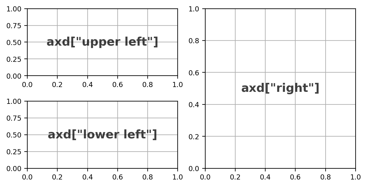
def annotate_axes(ax, text, fontsize): ax.text(0.5, 0.5, text, transform=ax.transAxes, alpha=0.75, ha="center", fontsize=fontsize, va="center", weight="bold")fig, axd = plt.subplot_mosaic([['upper left', 'right'], ['lower left', 'right']], figsize=(6,3), constrained_layout=True, dpi=200)for k in axd: annotate_axes(axd[k], f'axd["{k}"]', fontsize=14) axd[k].grid() |
除此之外,也可以使用其他的方法进行对子图的灵活布局,十分简单易用:
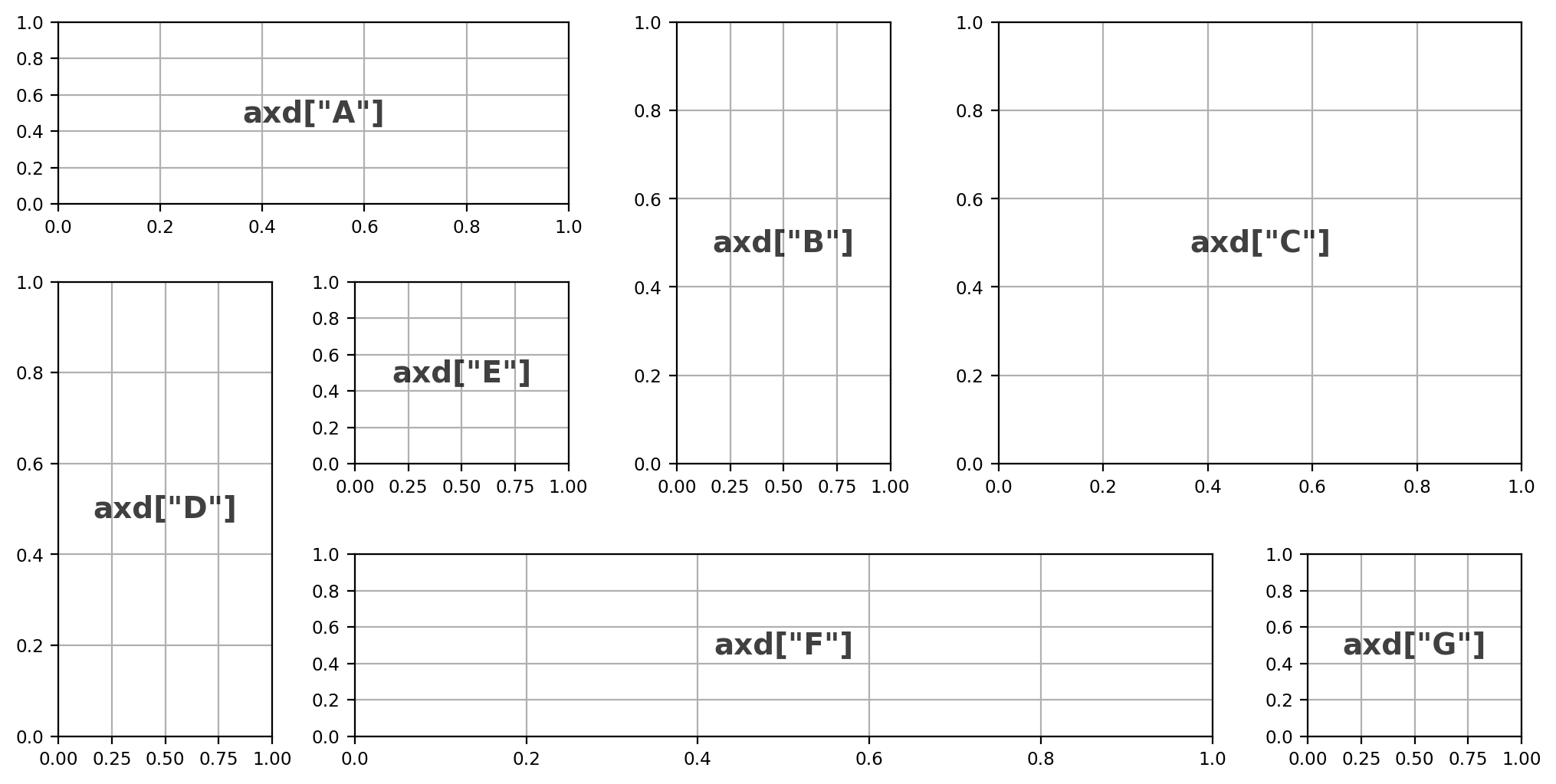
subplot_format = \"""AABCCDEBCCDFFFG"""fig, axd = plt.subplot_mosaic(subplot_format, figsize=(10, 5), constrained_layout=True, dpi=200)for k in axd: annotate_axes(axd[k], f'axd["{k}"]', fontsize=14) axd[k].grid() |
在原书中还有另一种使用嵌套列表的表示法,由于其不如格式字符串设置简便,在此暂且不加讨论。
1.6 常见的图类型
| 图类型 | 绘图函数 | 示例 |
|---|---|---|
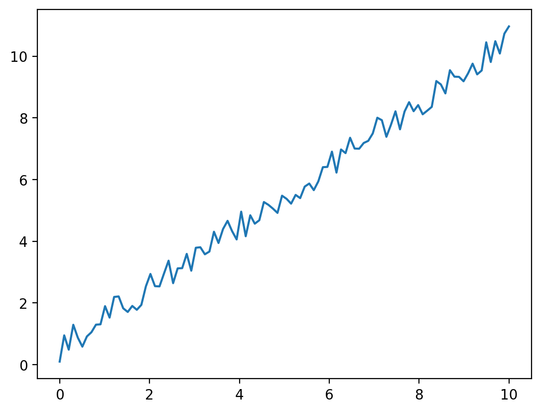
| 折线图 | plot |
 |
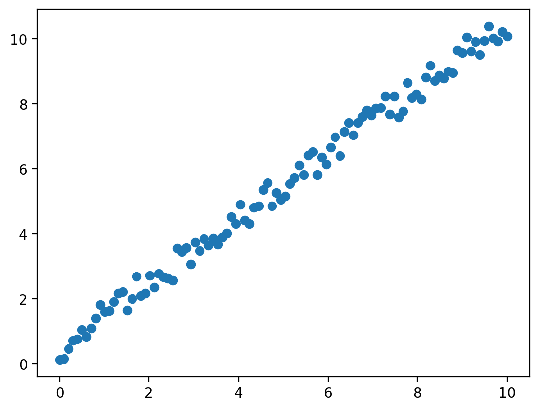
| 散点图 | scatter |
 |
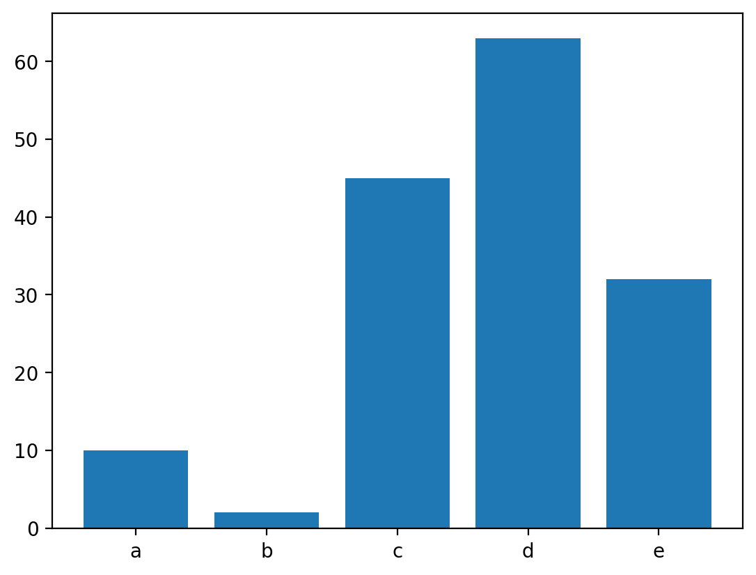
| 条形图 | bar / barh |
 |
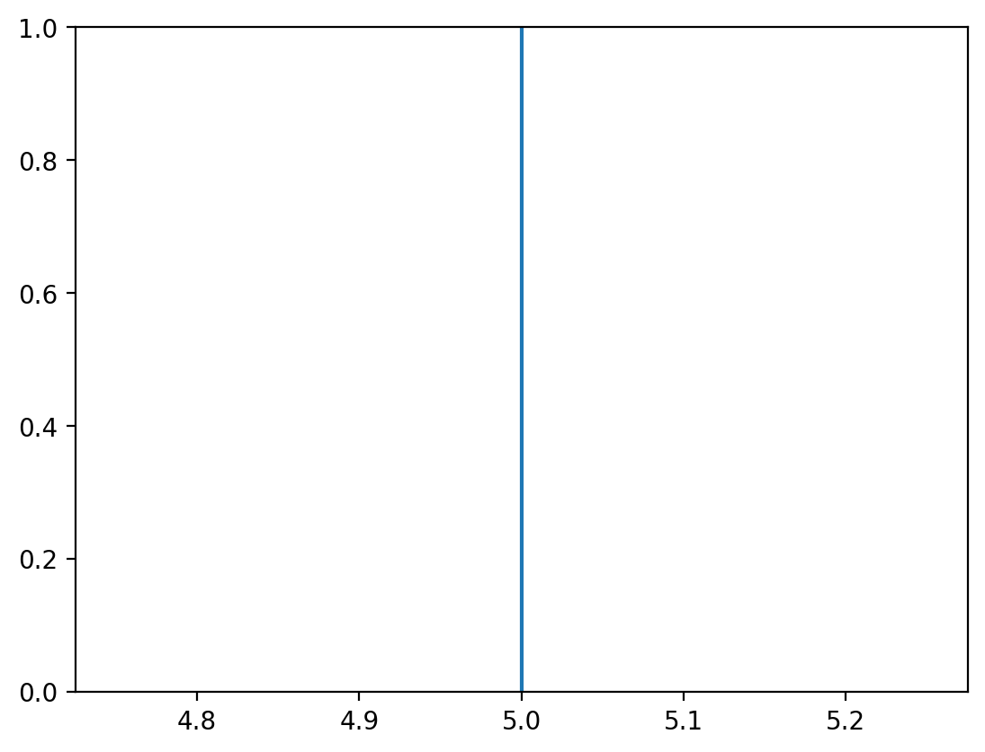
| 竖直线 | axvline |
 |
| 水平线 | axhline |
 |
| 与轴垂直的矩形 | axhspan / axvspan |
 |
| 文本 | text |
 |
| 填充 | fill_between |
 |
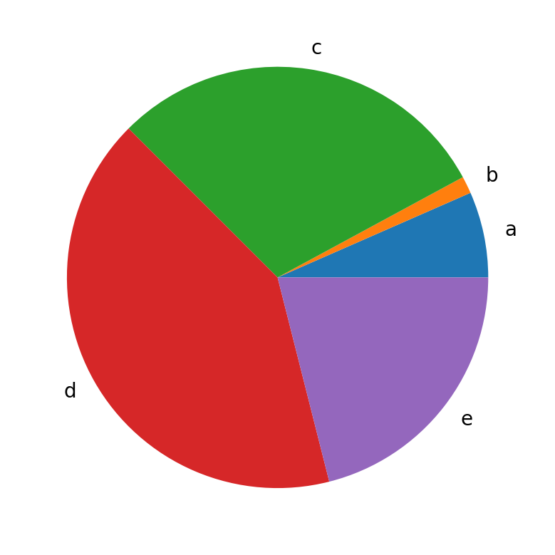
| 饼图 | pies |
 |
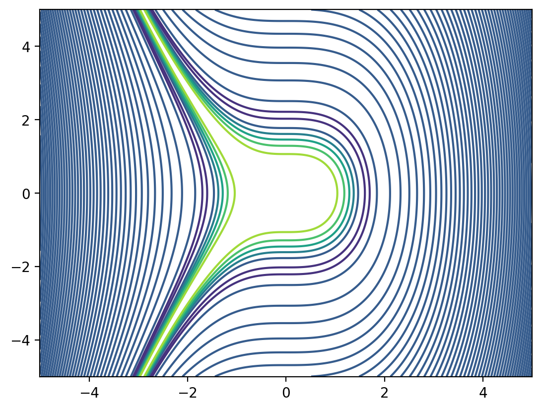
| 等高线图 | contour |
 |
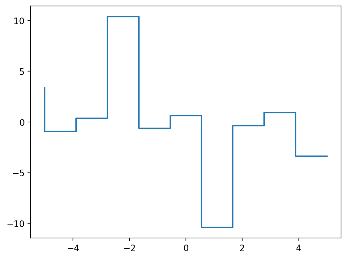
| 步阶图 | step |
 |
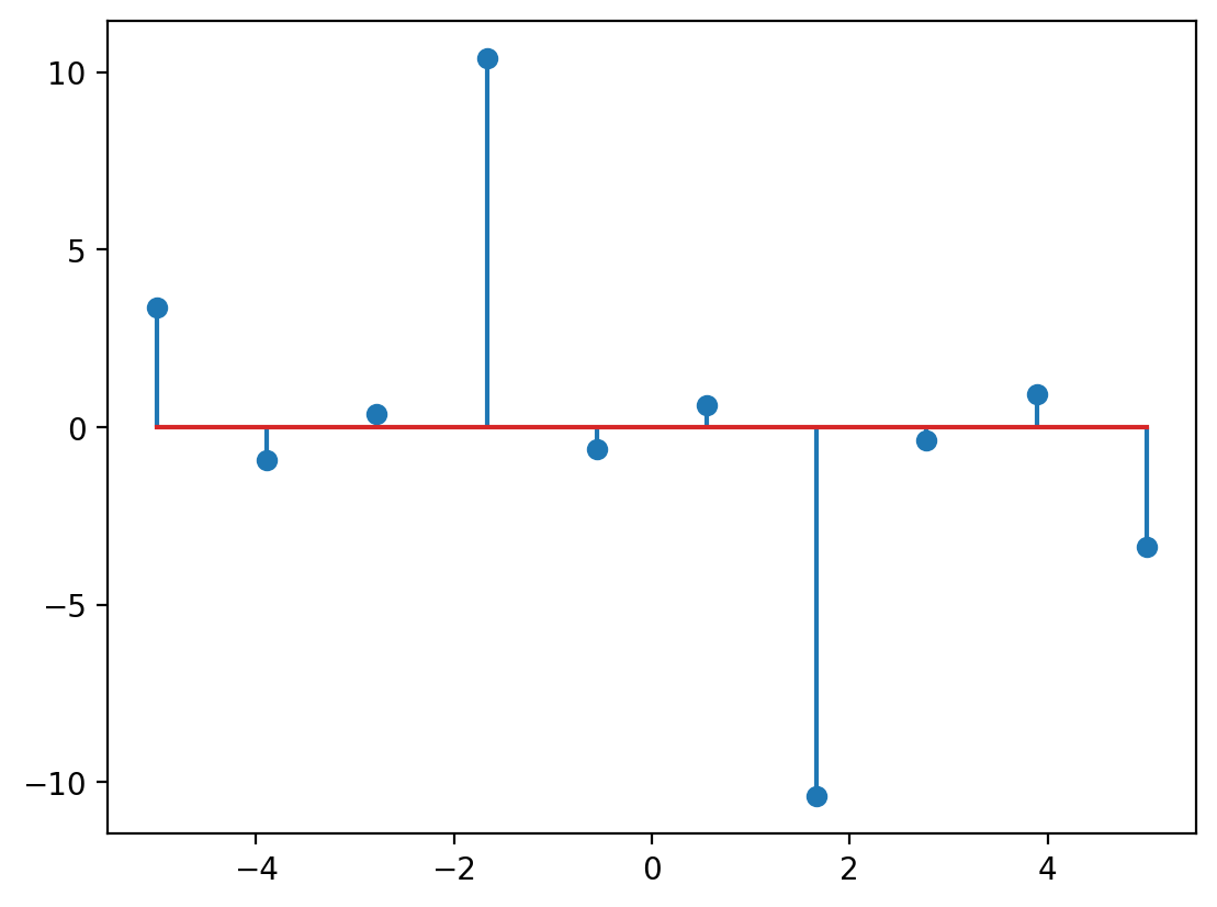
| 茎叶图 | stem |
 |
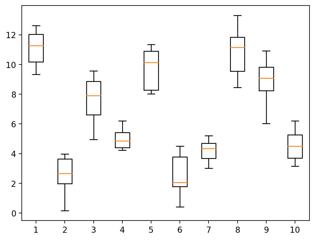
| 箱线图 | boxplot |
 |
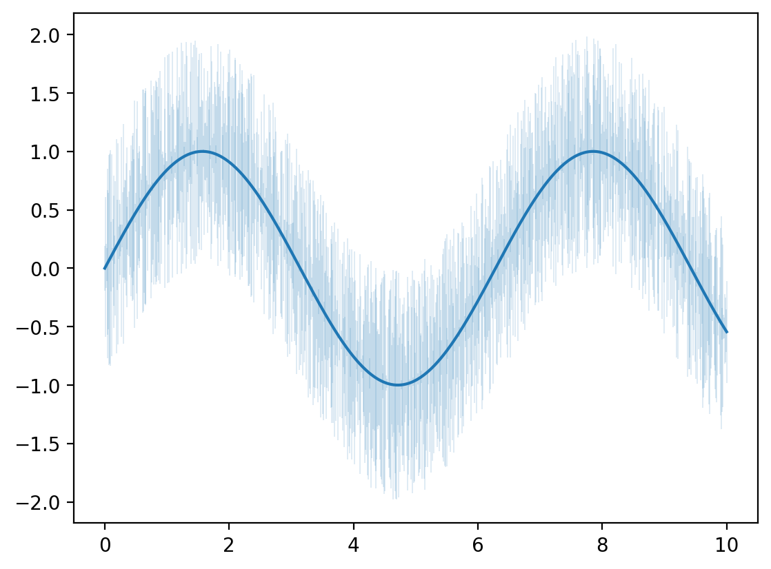
| 误差线 | errorbar |
 |
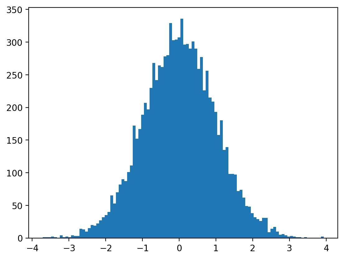
| 直方图 | hist |
 |
| 小提琴图 | violinplot |
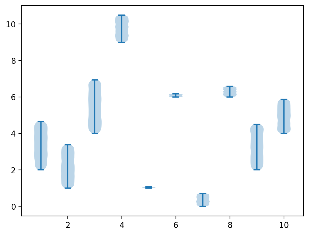 |
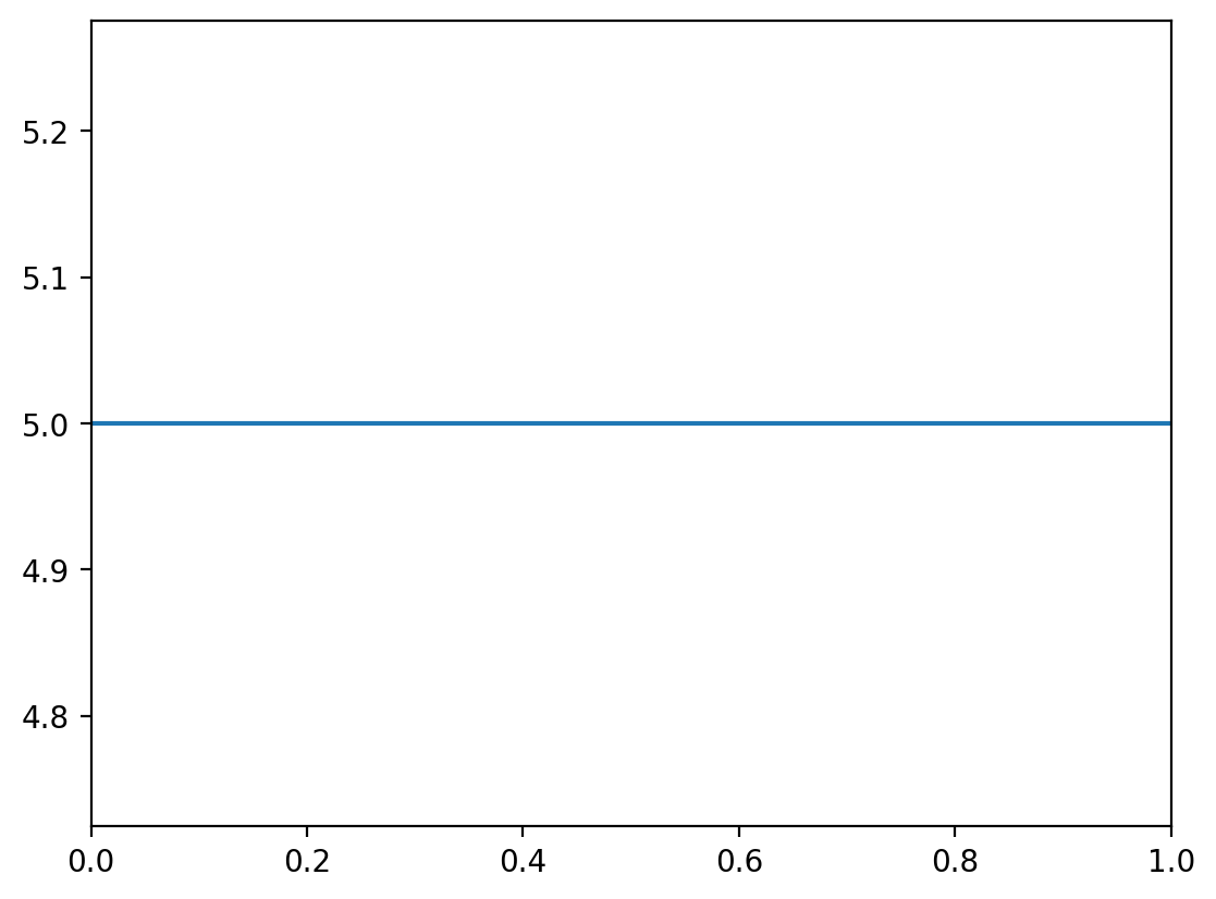
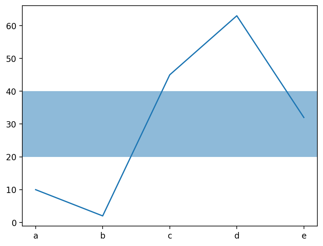
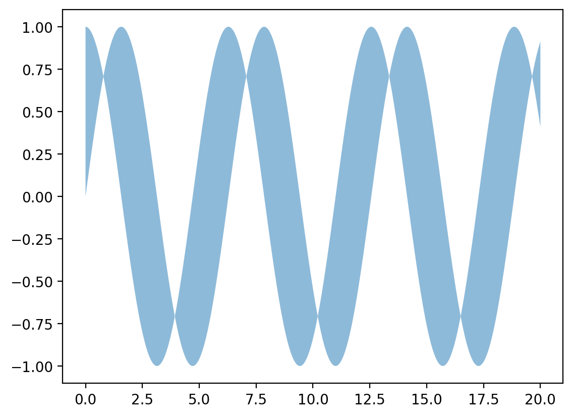
# plotx = np.linspace(0, 10, 100)y = x + np.random.rand(*x.shape)plt.figure(dpi=200)plt.plot(x, y)# scatterx = np.linspace(0, 10, 100)y = x + np.random.rand(*x.shape)plt.figure(dpi=200)plt.scatter(x, y)# barx = ['a', 'b', 'c', 'd', 'e']y = [10, 2, 45, 63, 32]plt.figure(dpi=200)plt.bar(x, y)# axvlineplt.figure(dpi=200)plt.axhline(5, 0, 10)# axhspanplt.figure(dpi=200)plt.axhspan(ymin=20, ymax=40, alpha=0.5)plt.plot(x, y)# textplt.figure(dpi=200)plt.text(0.5, 0.5, "Matplotlib", centeralign=True)# fill_betweenx = np.linspace(0, 20, 2000)y1 = np.sin(x)y2 = np.cos(x)plt.figure(dpi=200)plt.fill_between(x, y1, y2, alpha=0.5)# piesx = ['a', 'b', 'c', 'd', 'e']y = [10, 2, 45, 63, 32]plt.figure(dpi=200)plt.pie(y, labels=x)# contourx, y = np.linspace(-5, 5, 1000), np.linspace(-5, 5, 1000)xx, yy = np.meshgrid(x, y)z = np.sin(xx**3 + yy**2) / (xx**3 + yy**2)plt.figure(dpi=200)plt.contour(x, y, z)# stepx = np.linspace(-5, 5, 10)y = np.tan(x)plt.figure(dpi=200)plt.step(x, y)# stemx = np.linspace(-5, 5, 10)y = np.tan(x)plt.figure(dpi=200)plt.stem(x, y)# boxplotx = [np.random.randint(0, 10) + np.random.rand(10) * abs(np.random.rand(1) + 0.2) * 5 for i in range(10)]plt.figure(dpi=200)plt.boxplot(x)# errorbarx = np.linspace(0, 10, 1000)yerr = np.random.rand(*x.shape)y = np.sin(x)plt.figure(dpi=200)plt.errorbar(x, y, yerr=yerr, elinewidth=0.1)# histx = np.random.randn(10000)plt.figure(dpi=200)plt.hist(x, bins=100)# violinplotx = [np.random.randint(0, 10) + np.random.rand(10000) * abs(np.random.rand(1)) * 3\ for i in range(10)]plt.figure(dpi=200)plt.violinplot(x) |
1.7 结果的保存
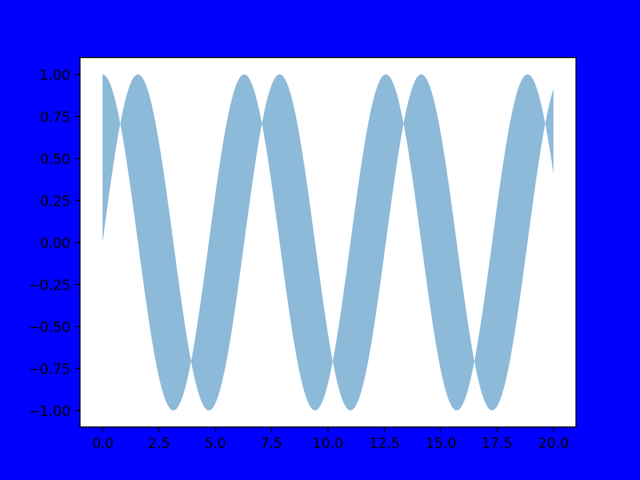
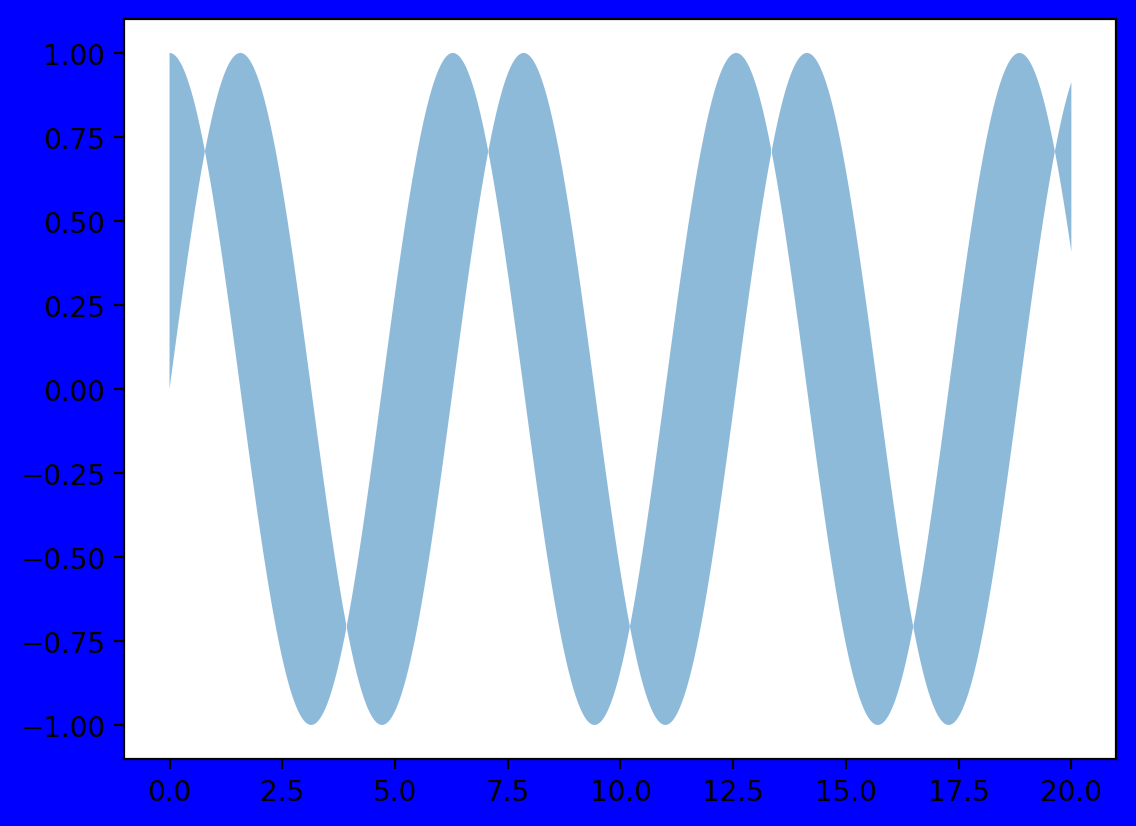
matplotlib可以将绘图结果存为多种格式,如PNG,JPG,TIFF,PDF,SVG等。使用savefig()函数保存画出的图像,这个函数需要在show之前,以避免保存图像为空白的问题。为去除图像四周的空白部分,可以设置bbox_inches="tight"来实现。以上文所述的fill_between函数的示例为例,分别指定和不指定bbox_tight参数,可以看出不指定参数(左)的四周空隙大于指定参数(右)的四周空隙。
x = np.linspace(0, 20, 2000)y1 = np.sin(x)y2 = np.cos(x)plt.figure(dpi=200, facecolor="blue")plt.fill_between(x, y1, y2, alpha=0.5)plt.savefig("./a.png")plt.savefig("./a_t.png", bbox_inches="tight") |