【Natural Language Processing】1 Word2vec (1)

Source: CS224n, Natural Language Processing with Deep Learning

1 Introduction to NLP

• complexity of communication enabled by language is a uniquely human intelligence among species
• Human children, interacting with a rich multi-modality world and various forms of feedback, acquire language with exceptional sample efficiency (not observing that much language) and compute efficiency (brains are efficient computing machines!)

A few applications of NLP

• Machine Translation
  • failures of these systems for most of the world’s 7000 languages, difficulties in translating long text, and ensuring contextual correctness of translations make this still a fruitful field of research.
• Question answering and information retrieval
• Summarization and analysis of text
  • NLP tools can be powerful for both the increase of access to information to the public, as well as surveillance, corporate or governmental.
• Speech-to-text

In all aspects of NLP, most existing tools work for precious few (usually one, maybe up to 100) of the world’s roughly 7000 languages, and fail disproportionately much on lesser-spoken and/or marginalized dialects, accents, and more. Beyond this, recent successes in building better systems have far outstripped our ability to characterize and audit these systems. Biases encoded in text, from race to gender to religion and more, are reflected and often amplified by NLP systems. With these challenges and considerations in mind, but with the desire to do good science and build trustworthy systems that improve peoples’ lives

2 Representing Words

2.1 Independent vectors for different words

• Simplest way to represent words is to use unrelated vectors (as a set)

Type is an element of a finite volcabulary
Token is an instance of a type observed in some context

We can store different words as independent standard basis (1-hot vector) of $\mathbb{R}^{n}$, i.e.

$$v_{\text{tea}} = e_{i} = \left[\, \begin{matrix} 0\\0\\1\\\vdots\\0 \end{matrix} \,\right], \quad v_{\text{coffee}} = e_{j} = \left[\, \begin{matrix} \vdots\\0\\1\\0\\\vdots \end{matrix} \,\right] .$$

We encode no similarity or relationship in this vectors, for different word vectors have inner product $0$:

$$\left\langle e_{i}, e_{j} \right\rangle = e_{i}^{\top} e_{j} \equiv 0,\quad i \ne j$$

and plus they are apparently not ordered.

2.2 Vectors from annotated discrete properties

We can construct word vector by the relationships that a word posess in the categories of grammar and other words.

$$v_{\text{tea}} = \left[ \, \begin{matrix} 0 \\ 0 \\ 1 \\ \vdots \\ 1 \end{matrix} \, \right] \begin{align*} & \rightarrow \text{plural noun}\\ & \rightarrow \text{3rd singular verb}\\ & \rightarrow \text{hyponym-of-beverage}\\ & \hspace{5em}\vdots\\ & \rightarrow \text{synonym-of-chai} \end{align*}$$

Failures of this method

1. Human annotated resources are always lacking in vocabulary compares to methods that can draw a vocabulary from a naturally occuring text source
2. A tradeoff between dimensionality and utility of the embedding—it takes a very high dimensional vector to represent all of these categories, which is costly and always incomplete.
3. Human ideas of what the right representations shoud be for text tend to underperform methods that allow data to determine more aspects

3 Distributional semantics and Word2vec

• We can learn rich representations of items using deep learning by means of unsupervised learning or (self-supervised learning)
• Unsupervised learning or self-supervised learning attempts to learning by predicting the remianing parts of data using unmasked parts.
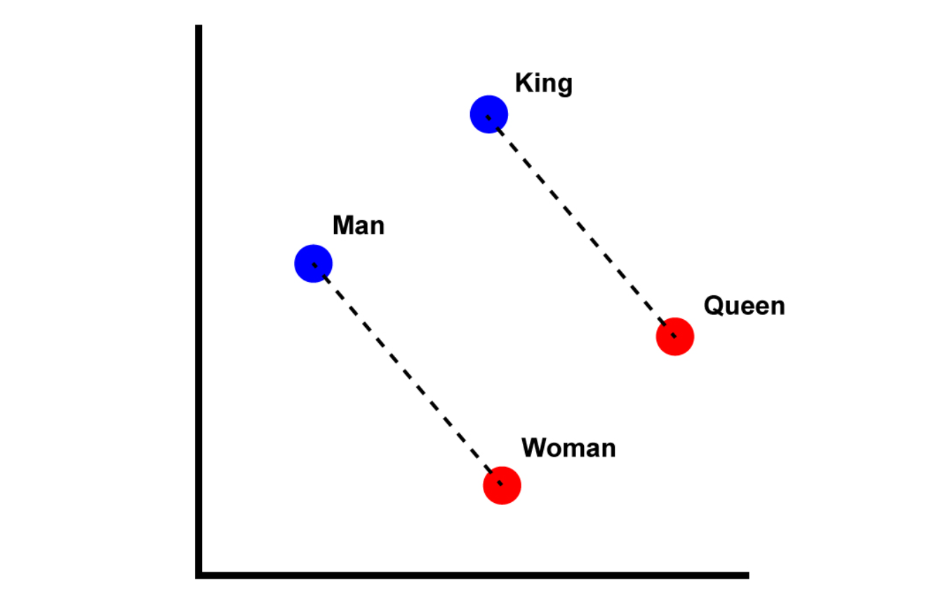
• You should know a word by the company it keeps.
• Words can be imagined as distributions over the semantic space where similar words appear nearer.

3.1 Co-occurrance matrices and document contexts

One idea of co-occurrance may be the following

1. Determine a vocabulary $\mathcal{V}$
2. Construct zero matrix of shape $|\mathcal{V}| \times |\mathcal{V}|$
3. Count the co-occurrances and fill in the matrix
4. Normalize rows by their sums

Assume the matrix is notated as $\boldsymbol{V}$, then word vectors of each word in vocabulary $\mathcal{V}$ is the rows of the matrix:

$$\boldsymbol{V} = \left[ \,\begin{matrix} v_{1}\\v_{2}\\ \vdots \\ v_{|\mathcal{V}|} \end{matrix}\, \right].$$

We can use various criterions to determine whether two words co-occurr, as the following shows:

$$\left[ \text{It's hot ans delicious.} \left[ \text{I pured} \left[ \text{the } \mathop{ \text{tea} }\limits_{ \blacktriangle } \text{ for} \right]_{\text{1}}\text{my uncle} \right]_{3} \right]_{\text{document}} ,$$

in which the subscripts of the brackets tells the radius of the co-ocurrance range and the black triangle indicates the central word tea.

Failures of this method

• Higher-dimensional vectors tend to be unwieldy
• Raw counts of co-occurrences over-emphasize the importance of common words such as the. Taking log frequency tend to be useful.
• Refer to GloVe (Pennington et al. 2014)

3.2 Word2vec

Skipgram word2vec model learns a short vector of words by peeking into a small contexts of words.

We have finite vocabulary $\mathcal{V}$, let $C,O \in \mathcal{V}$ be random variables representing unknown pair of words with $C$ representing center word and $O$ representing an outside word and let $c$ and $o$ represent specific values of corresponding values of these random variables.

Let $U, V \in \mathbb{R}^{|\mathcal{V}| \times d}$ be matrices and each word in $\mathcal{V}$ is associated in the corresponding row in $U$ and $V$.

Skipgram word2vec
The word2vec model is as follows

$$p_{U,V}(o|c) = \frac{\exp \left\{ u_{o}^{\top}v_{c} \right\}}{\sum\limits_{w \in \mathcal{V}} \exp \left\{ u_{w}^{\top} v_{c} \right\} },$$

in which $u_{w}$ refers to row of $U$ corresponding to word $w \in \mathcal{V}$. Note that $p_{U,V}(\cdot|c) \in \mathbb{R}^{|\mathcal{V}|}$
is the probabilites of all words given the center word $c$, which is similar to the row in the co-occurrance matrix $\boldsymbol{V}$.

Then we learn to optimize the cross-entropy loss with the true distribution $P^{*}(O|C)$:

$$\min_{U,V} \mathbb{E}_{O,C} \left[ -\log p_{U,V}(o|c) \right] = \min_{U,V} \sum_{o,c} -p^{*}(o|c)\log p(o|c).$$

Questions

• How do we perform the min operation?
• How do we get the random variables?
• Why the negative-log of the probability?
• Why is this much better than the co-occurrance counting?
• Why not all distributions over $o$ and $c$ can be represented by this model?

3.3 Estimating a word2vec model from a corpus

Word2vec empirical loss
Consider how we estimate the expectation term in the aforementioned model, we perform empirical loss. Let $D$ be a set of documents $\{ d_{i} \}_{i=1}$, where each contains a sequence of word $(w_{1}^{(d)}, \dots, w_{m}^{(d)})$ with all $w_{i}^{(d)} \in \mathcal{V}$ and let $k \in \mathbb{N}_{>0}$ be a positive-integer window size. For all center word $w_{i}$, we take the words within the window size, i.e. $\{ w_{i-k}, \dots, w_{i-1}, w_{i+1}, \dots, w_{i+k} \}$ to estimate the expectation term:

$$\begin{align} L(U,V) &= \sum\limits_{d \in D} \sum\limits_{i=1}^{m} \sum\limits_{j=1}^{k} -\log p_{U,V} \Big[w_{i-j}^{(d)} \Big| w_{i}^{(d)} \Big]\\ &= \sum\limits_{d \in D} \sum\limits_{i=1}^{m} \sum\limits_{j=1}^{k} -\log \left[ \frac{\exp \left\{ {w_{i-j}^{(d)}}^{\top}w_{i}^{(d)} \right\}}{\sum\limits_{s = 1}^{m} \exp \left\{ {w_{s}^{(d)}}^{\top} w_{i}^{(d)} \right\}} \right] . \end{align}$$

Gradient-based estimation
We first initialize the matrices $U$ and $V$ by drawing entries from gaussian distribution such as $\mathcal{N}(0, 1\times e^{-3})$ and preform gradient descent on $U$:

$$U \leftarrow U - \alpha \cdot \nabla_{U} L(U,V).$$

Stochastic gradient
Summing over the entire set of documents can be expansive, so we update matrix $U$ every time when having seen only as few of them:

$$\hat{L}(U,V) = \sum\limits_{d_{1},\dots,d_{l}} \sum\limits_{i=1}^{m} \sum\limits_{j=1}^{k} -\log p_{U,V} \Big[w_{i-j}^{(d)} \Big| w_{i}^{(d)} \Big]$$

for some integer $l \in \mathbb{N}_{>0}$.

3.4 Calculating gradient

By the linearity of gradient operator, we have

$$\begin{align} \nabla_{v_{c}} \hat{L}(U, V) &= \sum\limits_{d_{1},\dots,d_{l}} \sum\limits_{i=1}^{m} \sum\limits_{j=1}^{k} -\nabla_{v_{c}} \log p_{U,V} \Big[w_{i-j}^{(d)} \Big| w_{i}^{(d)} \Big]\\ &= \sum\limits_{d_{1},\dots,d_{l}} \sum\limits_{i=1}^{m} \sum\limits_{j=1}^{k} -{\color{blue} \nabla_{v_{c}} \left[ \log \frac{\exp \left\{ u_{o}^{\top}v_{c} \right\}}{\sum\limits_{w \in \mathcal{V}} \exp \left\{ u_{w}^{\top} v_{c} \right\} } \right] }. \end{align}$$

We can split the term in blue into two terms by the properties of log function and the linearity of gradient operator:

$$\begin{align} \nabla_{v_{c}} \left[ \log \frac{\exp \left\{ u_{o}^{\top}v_{c} \right\}}{\sum\limits_{w \in \mathcal{V}} \exp \left\{ u_{w}^{\top} v_{c} \right\} } \right] &= {\color{red} \nabla_{v_{c}} \log \exp \left\{ u_{o}^{\top}v_{c} \right\}} - {\color{blue} \nabla_{v_{c}} \log \sum\limits_{w \in \mathcal{V}} \exp \left\{ u_{w}^{\top} v_{c} \right\}}\\ &= {\color{red} u_{o}} + {\color{blue} \frac{1}{\sum\limits_{w \in \mathcal{V}} \exp \left\{ u_{w}^{\top} v_{c} \right\}}}\nabla_{v_{c}} \sum\limits_{w' \in \mathcal{V}} \exp \left\{ u_{w'}^{\top} v_{c} \right\} \\ & \hspace{1em}\small\text{(Inverse operation, Chain rule)}\\ &= {\color{red} u_{o}} + \frac{1}{\sum\limits_{w \in \mathcal{V}} \exp \left\{ u_{w}^{\top} v_{c} \right\}} {\color{blue} \sum\limits_{w' \in \mathcal{V}} \nabla_{v_{c}} } \exp \left\{ u_{w'}^{\top} v_{c} \right\} \\ & \hspace{1em}\small\text{(Lineararity of gradient op.)}\\ &= {\color{red} u_{o}} + \frac{1}{\sum\limits_{w \in \mathcal{V}} \exp \left\{ u_{w}^{\top} v_{c} \right\}} \sum\limits_{w' \in \mathcal{V}} {\color{blue} \exp \left\{ u_{w'}^{\top} v_{c} \right\} \nabla_{v_{c}} u_{w'}^{\top} v_{c} } \\ & \hspace{1em}\small\text{(Chain rule)}\\ &= {\color{red} u_{o}} + \frac{1}{\sum\limits_{w \in \mathcal{V}} \exp \left\{ u_{w}^{\top} v_{c} \right\}} \sum\limits_{w' \in \mathcal{V}} \exp \left\{ u_{w'}^{\top} v_{c} \right\} {\color{blue}u_{w'} } \\ \end{align}$$

When observing the second term, one can derive that

$$\begin{align} \frac{1}{\sum\limits_{w \in \mathcal{V}} \exp \left\{ u_{w}^{\top} v_{c} \right\}} \sum\limits_{w' \in \mathcal{V}} \exp \left\{ u_{w'}^{\top} v_{c} \right\} u_{w'} &= \sum\limits_{w' \in \mathcal{V}} \frac{\exp \left\{ u_{w'}^{\top} v_{c} \right\}}{\sum\limits_{w \in \mathcal{V}} \exp \left\{ u_{w}^{\top} v_{c} \right\}} u_{w'} \\ &= \sum\limits_{w' \in \mathcal{V}} p_{U,V}(w'|c) u_{w'}\\ &= \mathbb{E}[u_{w'}] \end{align}$$

Thus the whole gradient term can be simplified as

$$\nabla_{v_{c}}\hat{L}(U,V) = \mathop{u_{o}}\limits_{\text{observed}} - \mathop{\mathbb{E}[u_{w}]}\limits_{\text{expected}},$$

which is in align with the intuition: upgrade the word vector towards the opposite direction of the expectation.

3.5 Skip-gram with negative sampling (SGNS)

Notice that calculating the following softmax function can be expansive due to the denominator:

$$p_{U,V}(o|c) = \frac{ \exp \left\{ u_{o}^{\top}v_{c} \right\}}{\color{blue} \sum\limits_{w \in \mathcal{V}} \exp \left\{ u_{w}^{\top} v_{c} \right\} },$$

which normalizes the vector. The skip-gram model encourages $u_{o}$ and $v_{c}$ to be similar and $u_{w}$ and $v_{c}$ to be different:

$$\log \sigma(u_{o}^{\top}v_{c}) + \sum\limits_{w=1}^{k} \Big[ \log \sigma (-u_{w}^{\top} v_{c}) \Big],$$

where $u_{l}$ is drawn from some distribution $p_{\text{neg}}$.